Complex-valued Neural Networks
Dramsch, J. S., Lüthje, M., & Christensen, A. N. (2019). Complex-valued neural networks for machine learning on non-stationary physical data. arXiv preprint arXiv:1905.12321. |
||
Github: https://github.com/JesperDramsch/Complex-CNN-Seismic |
||

In the paper (Jesper Sören Dramsch, Lüthje, and Christensen 2019) I explore complex-valued deep convolutional networks to show that phase content in non-stationary data improves generalization of convolutional neural networks. This work implements self-supervised aes that compress the data and measure the reconstruction of the seismic data.
Four different deep convolutional aes are constructed. Two aes are real-valued and two aes are complex-valued. The complex-valued convolutional neural network is implemented as two real-valued feature maps, one for the real component \(a\) and one for the complex component \(b\) each, which are combined into a complex-valued number with \(a + b\text{i}\). The complex convolution is then implemented explicitly in the calculation to avoid some drawbacks of using complex numbers by a computer. However, matching the networks proved to be a complicated task with regard to the number of parameters. This led to building four different architectures that get progressively bigger and compare the results.
This study implements aes to increase the validity of this experiment. While vaes have shown better performance on reconstruction tasks, it would also introduce more variability in the network to control for. Considering that asi is a fairly new discipline, it is difficult to disambiguate effects on misclassification. These effects include erroneous labels, the difficulty of the task of asi, as well as the choice of architecture.
Therefore, this leads us to the decision to inspect the reconstructed seismic data numerically. Signal analysis is well-explored in the seismic data processing. Moreover, this enables analysing the result in the fk-domain providing additional insight to the denoising effect of the aes. Overall, the complex-valued networks result in smaller networks compared to a larger real-valued network achieving comparable reconstruction error.
Journal Paper: Complex-valued neural networks for machine learning on non-stationary physical data
Introduction
Seismic data has its caveats due to the complicated nature of bandwidth-limited wave-based imaging. Common problems are cycle-skipping of wavelets and nullspaces in inversion problems (Özdoğan Yilmaz 2001). Automatic seismic interpretation is complicated, as the modelling of seismic data is computationally expensive and often proprietary. Seismic field data is often not available and their interpretation is highly subjective and ground truth is not available. The lack of training data has been delaying the adoption of existing methods and hindering the development of specific geophysical deep learning methods. Incorporating domain knowledge into general deep learning models has been successful in other fields (Paganini, Oliveira, and Nachman 2017).
The state-of-the-art method has been an iterative windowed Fourier transform for phase reconstruction (Griffin and Lim 1984). Modern neural audio synthesis focuses on methods that do not require explicit reconstruction of the phase (Mehri et al. 2016; Oord et al. 2016, 2017; Prenger, Valle, and Catanzaro 2018). Mehri et al. (2016) introduced a recurrent neural network formulation, where Oord et al. (2016) reformulated the network for audio synthesis in a strided convolutional network. The original WaveNet formulation in Oord et al. (2016) is slow due to the autoregressive filter, warranting the parallel formulation in Oord et al. (2017).
We explicitly incorporate phase information in a deep convolutional neural network. These have been heavily explored in the digital signal processing community, before the recent renaissance of neural networks and deep learning. Relevant examples to seismic data processing include source separation (Scarpiniti et al. 2008), adaptive noise reduction (Suksmono and Hirose 2002), and optical flow (Miyauchi et al. 1993) with complex-valued neural networks. Sarroff (2018) gives a comprehensive overview of applications of complex-valued neural networks in signal and image processing.
In this work, we evaluate the reconstruction error after compression in an autoencoder to test how reliable information can be contained within a network with and without explicit phase information. This insight can be transferred to the aforementioned applications that benefit from an increase in information recovery. We calculate the complex-valued seismic trace by applying the Hilbert transform to each trace. Phase information has been shown to be valuable in the processing (Liner 2002) and interpretation of seismic data (Rocky Roden and Sepúlveda 1999; Mavko, Mukerji, and Dvorkin 2003). Steve Purves (2014) provides a tutorial that shows the implementation details of Hilbert transforms.
In this paper we give a brief overview of convolutional neural networks and then introduce the extension to complex neural networks and seismic data. We show that including explicit phase information provides superior results to real-valued convolutional neural networks for seismic data. Difficult areas that contain seismic discontinuities due to geologic faulting are resolved better without leakage of seismic horizons. We train and evaluate several complex-valued and real-valued autoencoders to show and compare these properties. These results can be directly extended to automatic seismic interpretation problems.
Complex Convolutional Neural Networks
Basic principles
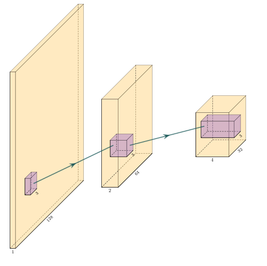
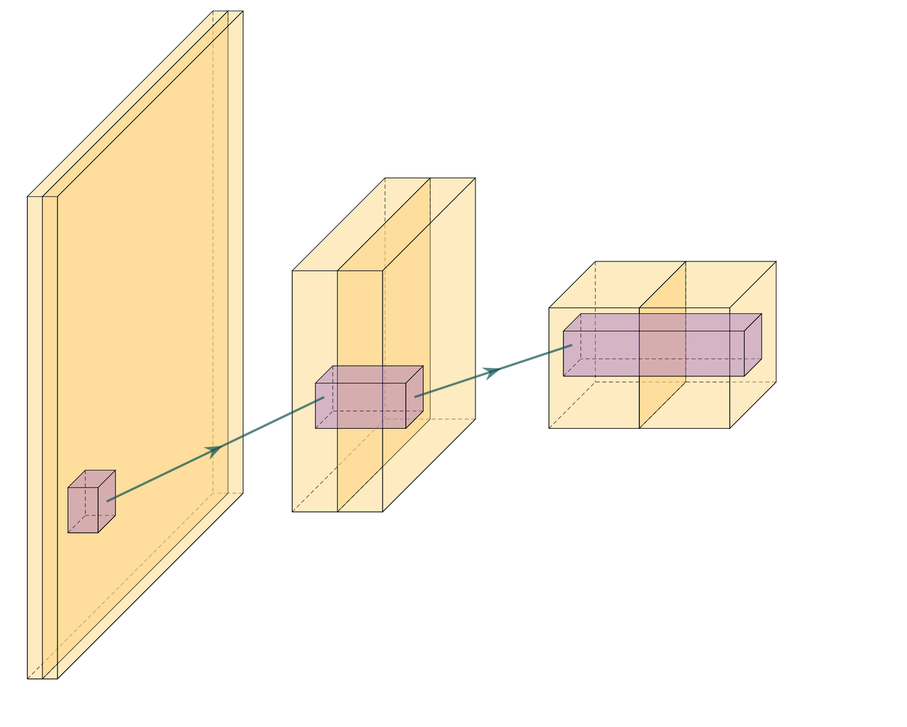
Convolutional neural networks (Y. LeCun et al. 1999) use multiple layers of convolution and subsampling to extract relevant information from the data (see Figure 5.1)
The input image is repeatedly convolved with filters and subsampled. This creates many, but smaller and smaller images. For a classification task, the final step is then a weighting of these very small images leading to a decision about what was in the original image. The filters are learned as part of the training process by exposing the network to training images. The salient point is, that the convolution kernels are learned based on the training. If the goal is - for example - to classify geological facies, the convolutional kernels will learn to extract information from the input, that helps with that task. It is thus a very strong methodology, that can be adapted to many tasks.
|
|
Figure 5.1: Schematic of equivalent real- and complex-valued convolutional neural networks. Yellow is the input image data and purple shows the 3 × 3 convolutional filters. In (a) the input image is convolved with filters. This results in several smaller outputs. The process is repeated, resulting in more outputs even further reduced in size. In (b) we present the complex-valued network. We start with a complex valued input represented by two layers, namely the real-valued a and complex-valued b complement in a+ib. The complex information is propagated through the network by keeping - in each step - the real and complex information in different layers after convolution with complex-valued filters.
Real- and Complex-valued Convolution
Convolution is an operation on two signals f and g or a signal and a filter that produce a third signal, containing information from both of the inputs. An example is the moving average filter, which smoothes the input, acting as a low-pass filter. Convolution is defined as
at the location \(\tau\). While often applied to real value signals, convolution can be used on complex signals. For the integral to exist both \(f\) and \(g\) must decay when approaching infinity. Convolution is directly generalizable to N-dimensions by multiple integrations and maintains commutativity, distributivity, and associativity. In digital signals this extends to discrete values by replacing the integration with summation.
Complex Convolutional Neural Networks
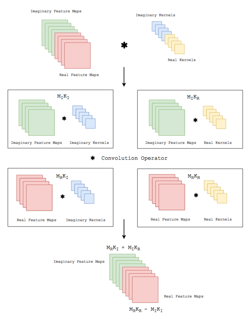
Implementation details of Complex Convolution (Courtesy Trabelsi et al. (2017))
Complex convolutional networks provide the benefit of explicitly modelling the phase space of physical systems (Trabelsi et al. 2017). Unfortunately it is not possible to feed complex numbers directly to a CNN, as they are not supported by any of the standard implementations (PyTorch or Tensorflow). Instead, we can represent them in another form. The complex convolution introduced in Section 3.1.2.2, can be explicitly implemented as convolutions of the real and complex components of both kernels and the data. A complex-valued data matrix in cartesian notation is defined as \(\textbf{M} = M_\Re + i M_\Im\) and equally, the complex-valued convolutional kernel is defined as \(\textbf{K} = K_\Re + i K_\Im\). The individual coefficients \((M_\Re, M_\Im, K_\Re, K_\Im)\) are real-valued matrices, considering vectors are special cases of matrices with one of two dimensions being one.
Solving the convolution of
we can apply the distributivity of convolutions (cf. section 5.1.2.2) to obtain
where \(K\) is the Kernel and \(M\) is a data vector (see Figure 5.1).
We can reformulate this in algebraic notation
Complex convolutional neural networks learn by back-propagation. Sarroff, Shepardson, and Casey (2015) state that the activation functions, as well as the loss function must be complex differentiable (holomorphic). Trabelsi et al. (2017) suggest that employing complex losses and activation functions is valid for speed, however, refers that Hirose and Yoshida (2012) show that complex-valued networks can be optimized individually with real-valued loss functions and contain piecewise real-valued activations. We reimplement the code Trabelsi et al. (2017) provides in keras (Chollet and others 2015a) with tensorflow (Abadi et al. 2015a), which provides convenience functions implementing a multitude of real-valued loss functions and activations.
While common up- and downsampling functions like MaxPooling, UpSampling, or striding do not suffer from complex-valued neural networks, batch normalization (BN) (Ioffe and Szegedy 2015) does. Real-valued batch normalization normalizes the data to zero mean and a standard deviation of 1. This does not guarantee normalization in complex values. Trabelsi et al. (2017) suggest implementing a 2D whitening operation as normalization in the following way.
where \(x\) is the data and \(V\) is the 2x2 covariance matrix, with the covariance matrix being
Effectively, this multiplies the inverse of the square root of the covariance matrix with the zero-centred data. This scales the covariance of the components instead of the variance of the data (Trabelsi et al. 2017).
Autoencoders
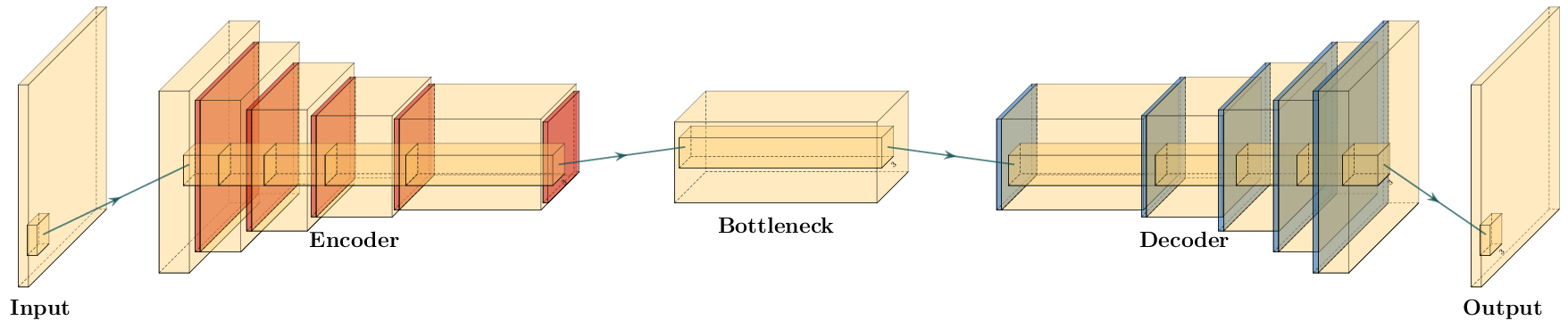
Typical autoencoder architecture. The data is compressed to a low dimensional bottleneck, and then reconstructed. In the encoder convolutional layers (yellow) are followed by a down-sampling operation (red) to reduce the spatial extend of the input image. The bottleneck contains a lower-dimensional compressed representation of the input. The decoder contains upsampling operations (blue) followed by convolutional layers symmetrical to the encoder. Alternatively, the encoder is sometimes made up of transpose convolutions.
Autoencoders (Hinton and Salakhutdinov 2006) are a special configuration of the encoder-decoder network that map data to a low-level representation and back to the original data. This low-level representation - the latent space - is often called bottleneck or code layer. Autoencoder networks map \(f(x) = x\), where \(x\) is the data and \(f\) is an arbitrary network. The architecture of autoencoders is an example of lossy compression and recovery from the lossy representation. Commonly, recovered data is blurred by this process.
The principle is illustrated in Figure 5.2. The input is transformed to a low-dimensional representation - called a code or latent space - and then reconstructed again from this low dimensional representation. The intuition is, that the network has to extract the most salient parts from the data, to be able to perform a reconstruction. As opposed to other methods for dimensionality reduction - e.g. principal component analysis - an autoencoder can find a non-linear representation of the data. The low-dimensional representation can then be used for anomaly detection, or classification.
Aliasing in Patch-based training
Mean-Shift in Neural Networks
A single neuron in a neural network can be described by \(\sigma ( w \cdot x + b )\), where \(w\) is the network weights, \(x\) is the input data, \(b\) is the network bias, and \(\sigma\) is a non-linear activation function. During training, the network weights \(w\) and biases \(b\) are are adjusted to a value that represents the training minimum. Learning on a mean-shift of \(q\) of an arbitrary distribution over \(x\) leads to \(\sigma( w \cdot (x + q) + b )\), which increases the neuron response by \(q\), weighted by \(w\). During inference, both \(w\) and \(b\) are fixed, by extension the mean-shift \(q\) is fixed as well. The mean-shift over larger inference data disappears, introducing an additional bias of \(w \cdot q\) before non-linear activation. This training bias may lead to prediction errors of the neuron and consequently the full neural network.
Windowed Aliasing
Non-stationary data such as seismic data can contain sections within the data that contain spurious offsets from the mean. Figure 5.3 shows varying sizes of cutouts, with 101 and 256 samples respectively. In the middle, the full normalised amplitude spectra are presented. On the right, the corresponding phase spectra are presented. On the left, we focus on the frequency content of the amplitude spectra around 0 Hz. The cutouts were Hanning tapered, however, a mean shift appears for any patch size.
These concepts of mean-shift corresponds to a DC offset in spectral data, which can be audio, seismic or electrical data. In images this corresponds to a non-zero alpha channel. While batch normalization can correct the mean shift in individual mini-batches (Ioffe and Szegedy 2015), this may shift the entire spectrum by the aliased offset. Additionally, batch normalization may not be feasible in some physical applications pertaining to regression tasks.
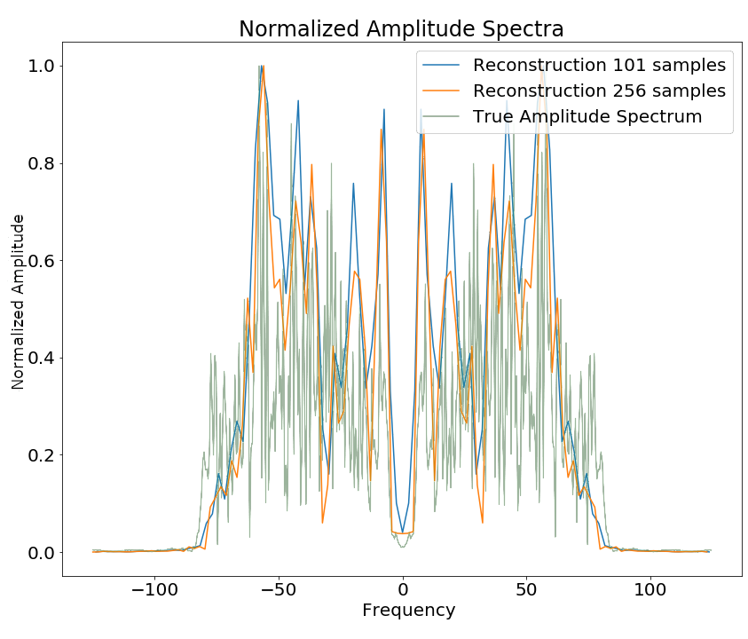
Spectral aliasing dependent on window-size (modified from Jesper Sören Dramsch and Lüthje (2018d)). The true amplitude spectrum (green) is 0 at a frequency of 0 Hz, whereas windows of the data experience low-frequency aliasing that introduce a non-zero offset at 0 Hz analogous to the Nyquist-Shannon theorem for high frequencies.
Complex Seismic Data
Complex seismic traces are calculated by applying the Hilbert transform to the real-valued signal. The Hilbert transform applies a convolution with to the signal, which is equivalent to a -90-degree phase rotation. It is essential that the signal does not contain a DC component, as this would not have a phase rotation.
The Hilbert transform is defined as
of a real-valued time series \(u(t)\), where the improper integral has to be interpreted as the Cauchy principal value. In the Fourier domain, the Hilbert transform has a convenient formulation, where frequencies are set zero and the remaining frequencies are multiplied by 2. This can be written as
where \(x_a\) is the analytical signal, \(x\) is the real signal, \(F\) is the Fourier transform, and \(U\) is the step function. The imaginary component \(y\) is simultaneously the quadrature of the real-valued trace. This provides locality to explicit phase information, where the Fourier transform itself does not lend itself to the resolution of the phase in the time domain. In conventional seismic trace analysis, the complex data is used to calculate the instantaneous amplitude and instantaneous frequency. These are beneficial seismic attributes for interpretation (Barnes 2007).
Experiments
Data
The data is the F3 seismic data, acquired in the Dutch North Sea in 1987 over an area of 375.31 km2. The sampling-rates are 4 ms in time and inline/crossline bins of 25 m. The extent being 650 inline traces and 950 crossline traces with a total length of 1.848 s. The data contains faulted reflector packets, of which the lowest one overlays a salt diapir. The data contains some noise that masks lower-amplitude events.
We generate 2D patches of size 64x64 in the inline and crossline direction from the 3D volume to train our network. We obtain inline and crossline 64x64 patches that are taken overlapping with a stride of 8 samples. The total amount of data is 188736 patches with 141552 for training and 47184 for validation in a 75/25 train-validation split. The test data is the holdout Alaudah et al. (2019) stored in test_once. The seismic data is normalized to values in the range of [-1, 1]. To obtain complex-valued seismic data we apply a Hilbert transform to every trace of the data and subtract the real-valued seismic from the real component as laid out in Taner, Koehler, and Sheriff (1979).
Architecture
Layer |
Spatial |
Complex |
Real |
Complex |
Real |
|
(Size) |
X |
Y |
Small |
Small |
Large |
Large |
Input |
64 |
64 |
2 |
1 |
2 |
1 |
CConv2D |
64 |
64 |
8 |
8 |
16 |
16 |
CConv2D + BN |
64 |
64 |
8 |
8 |
16 |
16 |
Pool + CConv2D + BN |
32 |
32 |
16 |
16 |
32 |
32 |
Pool + CConv2D + BN |
16 |
16 |
32 |
32 |
64 |
64 |
Pool + CConv2D + BN |
8 |
8 |
64 |
64 |
128 |
128 |
Pool + CConv2D |
4 |
4 |
128 |
128 |
256 |
256 |
Up + CConv2D + BN |
8 |
8 |
64 |
64 |
128 |
128 |
Up + CConv2D + BN |
16 |
16 |
32 |
32 |
64 |
64 |
Up + CConv2D + BN |
32 |
32 |
16 |
16 |
32 |
32 |
Up + CConv2D |
64 |
64 |
8 |
8 |
16 |
16 |
CConv2D |
64 |
64 |
8 |
8 |
16 |
16 |
CConv2D |
64 |
64 |
2 |
1 |
2 |
1 |
Par ameters on Graph |
100,226 |
198,001 |
397,442 |
790,945 |
||
Comp ression Ratio |
4:1 |
2:1 |
2:1 |
1:1 |
||
Size on Disk [MB] |
1.4 |
2.5 |
4.8 |
9.2 |
The autoencoder architecture compresses the input data to a lower dimensional representation, i.e. bottleneck (cf. Figure 5.2), with an encoder network and reconstruct the input data from the bottleneck with a decoder network. It is common that the encoder and decoder networks are formulated symmetrically, as we have done in this paper. We reduce a 64x64 input 4 times by a factor of two spatially to encode a 4x4 encoding layer. We define varying amounts of filters during the downsampling steps and in the code layer to achieve varying amounts of compression shown in Table 5.1. The architecture for the complex convolutional network is identical to the real network, except for replacing the real-valued 2D convolutions with complex-valued convolutions represented by two feature maps instead of one. The layers for each network are shown in Table 5.1 with additional values, including learnable parameters counted on the computational graph, compression ratio, and size on disk. In total four network architectures are presented, two real-valued and complex-valued networks each matched in the number of feature maps, resulting in different amounts of parameters and compression ratio. The parameters are counted on the computational graph compiled by Tensorflow.
The neural networks specifically use 2D convolutions with 3x3 kernels. We employ batch normalization to regularize and speed up training (Ioffe and Szegedy 2015). The down and up sampling is achieved by MaxPooling and the UpSampling operation respectively.
Complex-valued neural networks contain two feature maps for every feature map contained in a real-valued network. Conceptually, this is equivalent to \(a + \text{i}b\), with \(b=0\) for the real-valued network. The information in the complex complement for these two feature maps is derived from the input data using the Hilbert transform. Following the argument of deep learning, this input could be derived from a neural network directly and should not provide an improvement to the networks reconstruction error. We define a complex-valued network that has the same number of filters as the real-valued network in both the "small" and "large" formulation in Table 5.1. This network effectively has half the available feature maps for the real-valued seismic input, as the other half is used for the complex-valued information. That means the smaller real-valued network contains as many feature maps for the real-valued seismic as the large complex network, the large real-valued network contains an additional feature map for every real-valued input for the complex component.
Training
We train the networks with an Adam optimizer (Diederik P. Kingma and Ba 2014) and a learning rate of \(10^{-3}\) without decay, for 100 epochs. The loss function is mean squared error, as the seismic data contains values in the range of [-1,1]. All networks reach stable convergence without overfitting, shown in Figure 5.4.
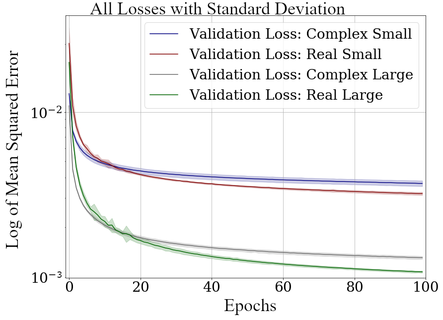
Validation Loss (MSE) on 7 random seeds per network. (Real-valued loss on real-valued seismic and combined complex-valued loss on complex-valued seismic, as the network "sees" it.)
Evaluation
We compare the complex autoencoders with the real-valued autoencoders, through the reconstruction error on unseen test data on 7 individual realizations of the respective four networks and qualitative analysis of reconstructed images. We focus on evaluating the real-valued reconstruction of the seismic data for both networks.
Results
We trained four neural network autoencoders with seven random initializations for each network, to allow for error bars on the estimates in Figure 5.4. The mean squared error and the mean absolute error for each parameter configuration during training is given in Table 5.2. There is a clear correspondence of the reconstruction error of the autoencoder to the size of network. The real-valued networks outperform the complex-valued networks in both the mean squared error and mean absolute error, however, we see that a real-valued network needs around twice as many parameters as a complex-valued network to attain the same reconstruction errors.
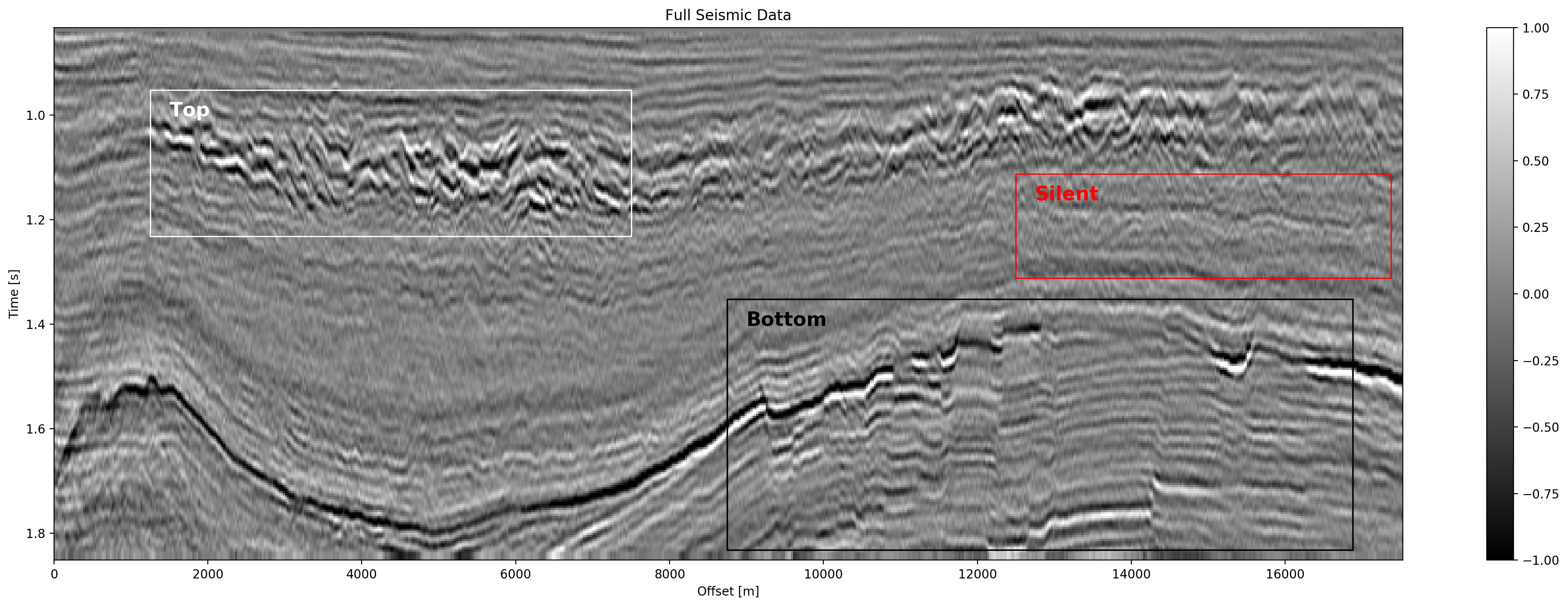
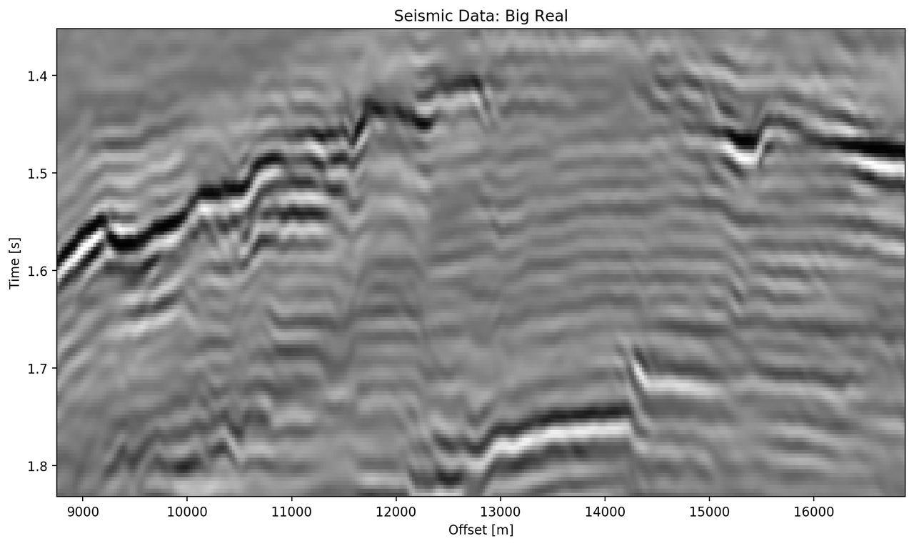
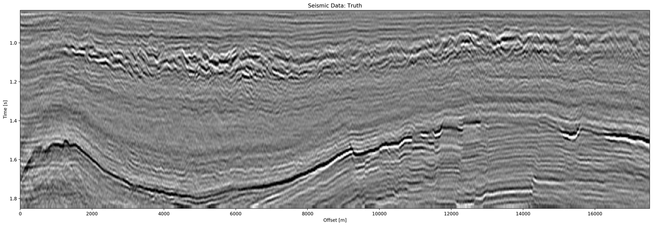
Seismic Test Data with marked section for closer inspection. We chose the "top" section for it’s faulted chaotic texture, "bottom" for the faulted blocks, and "silent" for a noisy but geologically uninteresting section.
Network |
Compression |
Parameters |
MSE [x10^-2] |
MAE [x10^-2] |
|---|---|---|---|---|
|
4:1 |
100,226 |
0.484 ± 0.013 |
4.695 ± 0.058 |
|
2:1 |
198,001 |
0.436 ± 0.006 |
4.500 ± 0.028 |
|
2:1 |
397,442 |
0.227 ± 0.003 |
3.247 ± 0.025 |
|
1:1 |
790,945 |
0.196 ± 0.002 |
3.050 ± 0.013 |
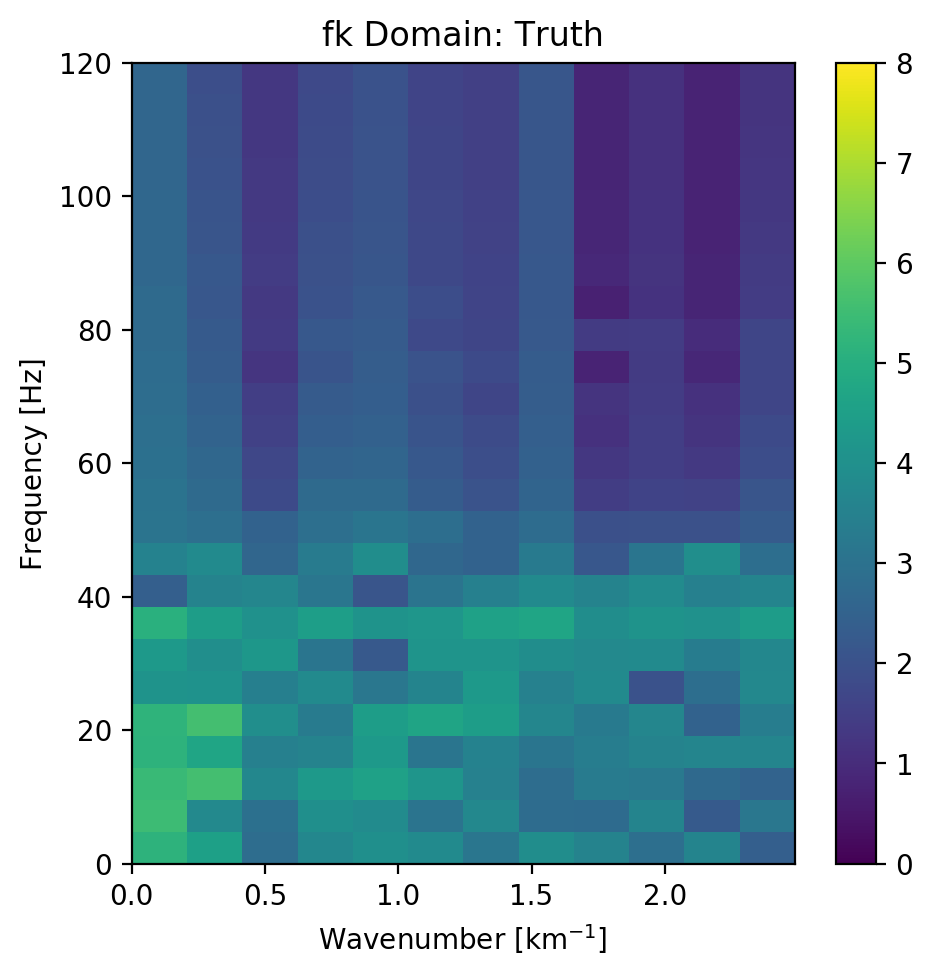
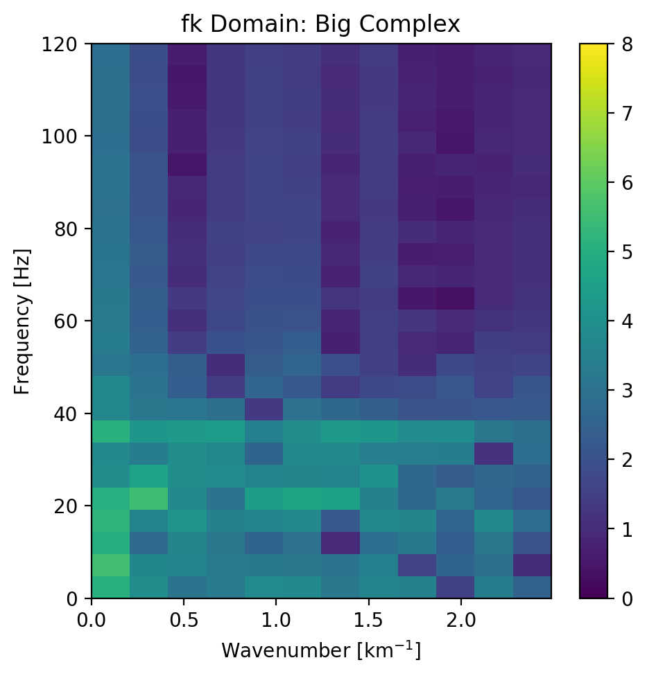
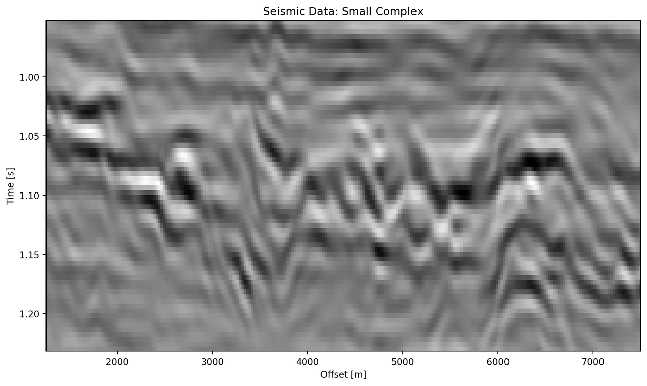
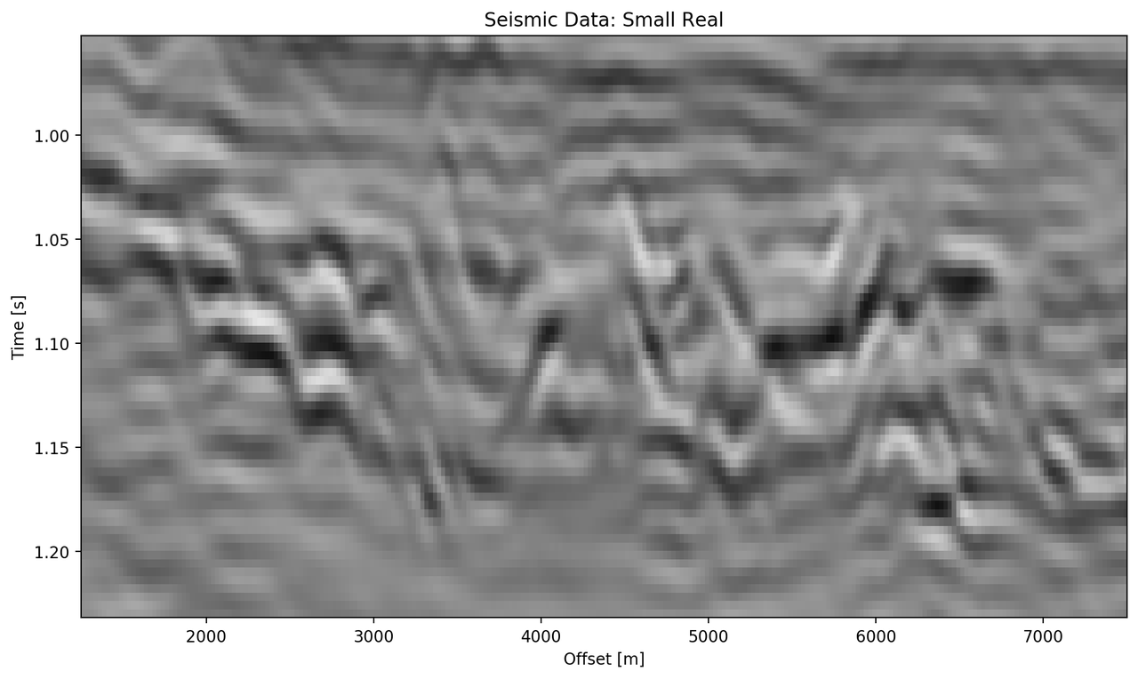
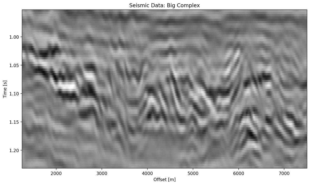
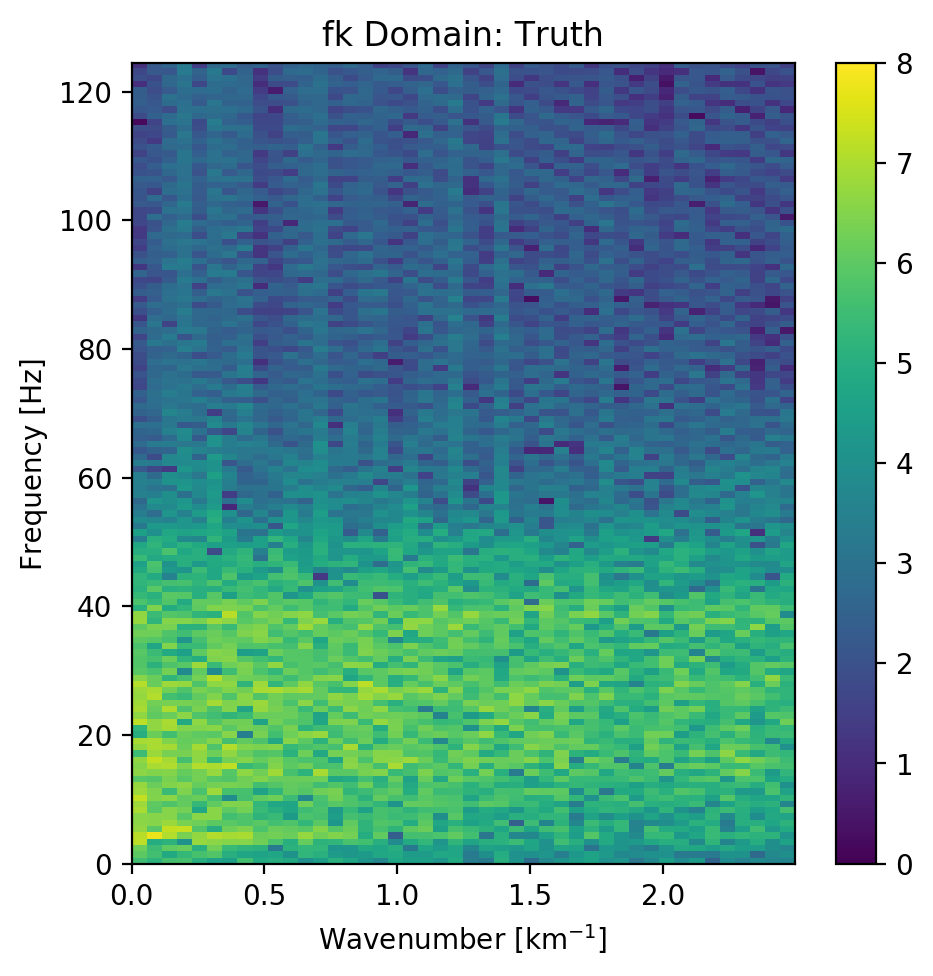
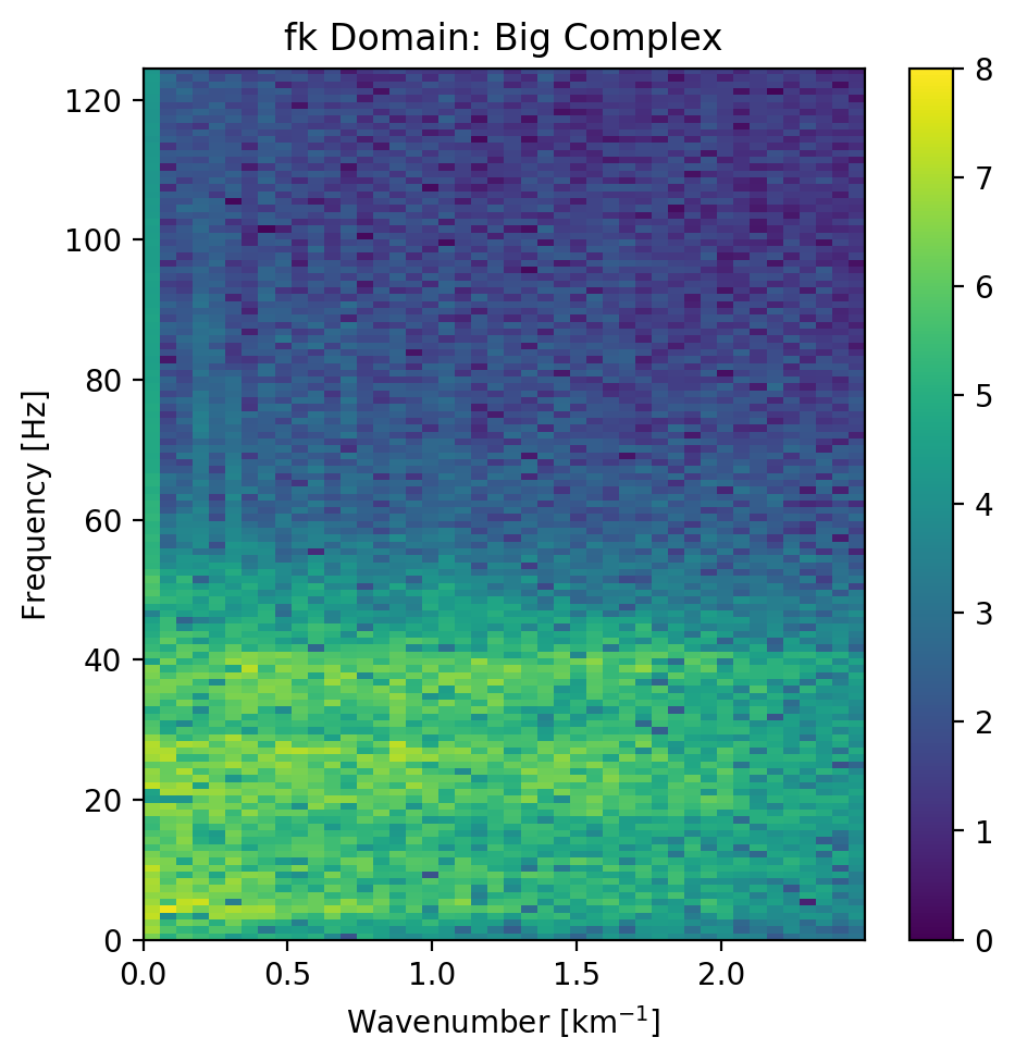
The seismic sections in Figure 5.5 show the unseen test seismic section. We perform a closer inspection of the regions "top" and "bottom" to focus on geologically relevant sections in the reconstruction process. The noisy segment without strong reflectors is a good baseline to evaluate the noise reduction of the autoencoder and the behaviour of the different networks on low amplitude data. Overall, all networks denoise the original seismic, with the lowest reconstruction errors being root-mean-squared (RMS) of 0.1187 and MAE of 0.0947 (cf. Table 5.3). Figure 5.7 shows the frequency-wavenumber (FK) of the ground truth (Figure 5.7 (a) ) and the large complex network reconstruction (Figure 5.7 (b) ). These show a decrease in the 0 - 60 Hz band for larger absolute wavenumbers.
Full |
Silent |
Top |
Bottom |
|||||
Network |
RMS |
MAE |
RMS |
MAE |
RMS |
MAE |
RMS |
MAE |
C_small |
0.1549 |
0.1145 |
0.1265 |
0.1010 |
0.2315 |
0.1759 |
0.1588 |
0.1200 |
R_small |
0.1581 |
0.1153 |
0.1247 |
0.0994 |
0.2395 |
0.1810 |
0.1612 |
0.1205 |
C_big |
0.1508 |
0.1101 |
0.1187 |
0.0947 |
0.2301 |
0.1747 |
0.1514 |
0.1135 |
R_big |
0.1469 |
0.1072 |
0.1214 |
0.0967 |
0.2222 |
0.1679 |
0.1459 |
0.1088 |
|
|
Figure 5.7: Evaluation on Silent Noise Patch in FK Domain. Noise reduction of frequencies below 50~Hz apparent, while reconstruction does not introduce visible aliasing.
"Top" seismic section
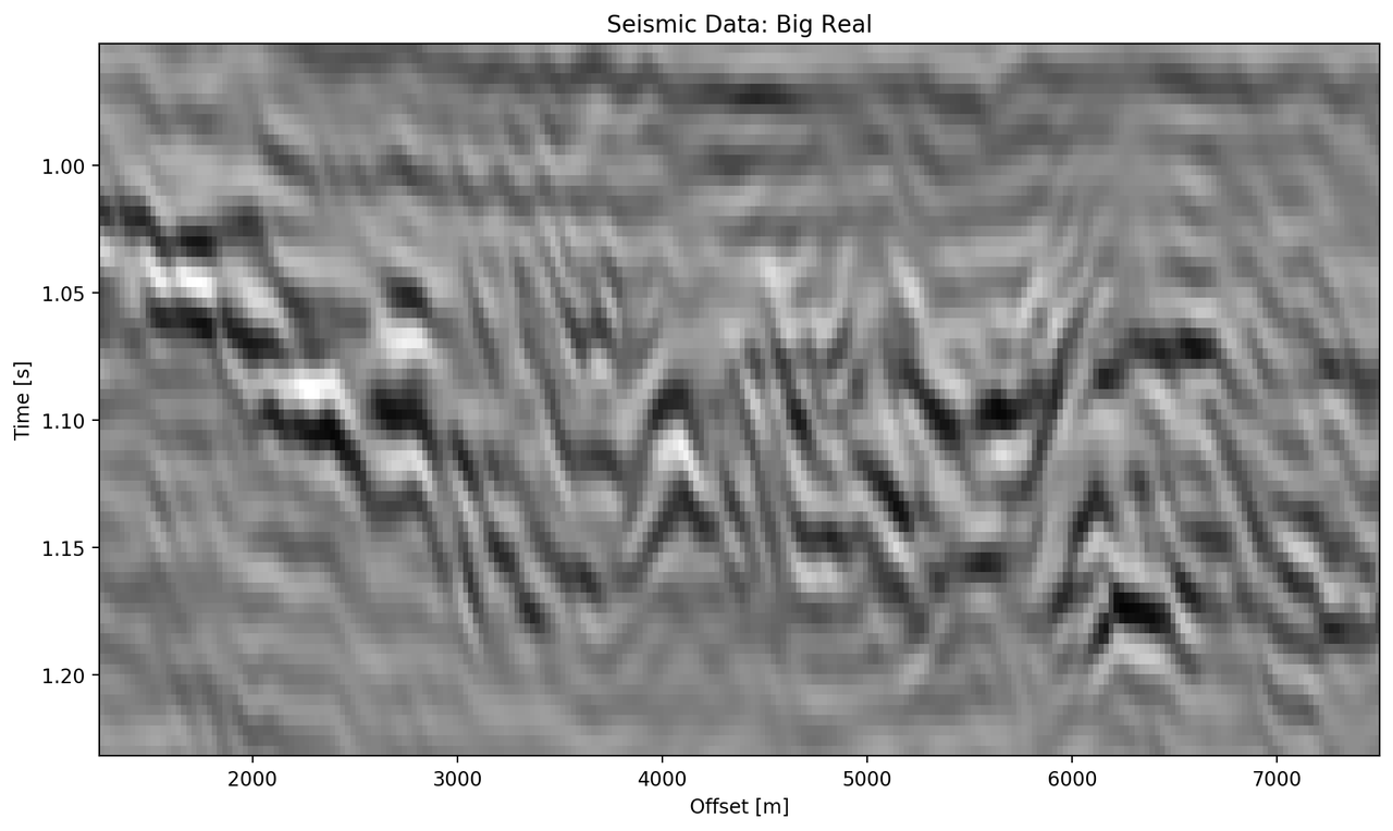
The "top" segment contains strong reflections that are very faulted with strong reflectors. Figure 5.8 shows the top segment and the reconstructions of the four networks. All networks display various amounts of smoothing. The quantitative results show that the complex networks perform very similar regardless of size. The large real-valued network outperforms the complex networks by 2.5 % on RMS, while the small real-valued network underperforms by 2.5 % on RMS. The panel in Figure 5.8 (c) shows a very smooth result. Despite the close score of the complex networks, it appears that the complex-valued network restores more high-frequency content. We can also see less smearing of discontinuities in the larger complex network, particularly visible in the lower part (1.2 s) at 6000 m offset, which is smeared to appear like a diffraction in the smaller network. The large real-valued network shows good reconstruction with minor smearing with higher amplitude fidelity in areas like 1.1 s at 2000 m, however, some of the steeply dipping artifacts are visible below the reflector packet between 0 m and 2000 m offset.

|
|
|
|
|
|
Figure 5.8: Evaluation on Top Noise Patch. Data is normalized between -1 and 1.
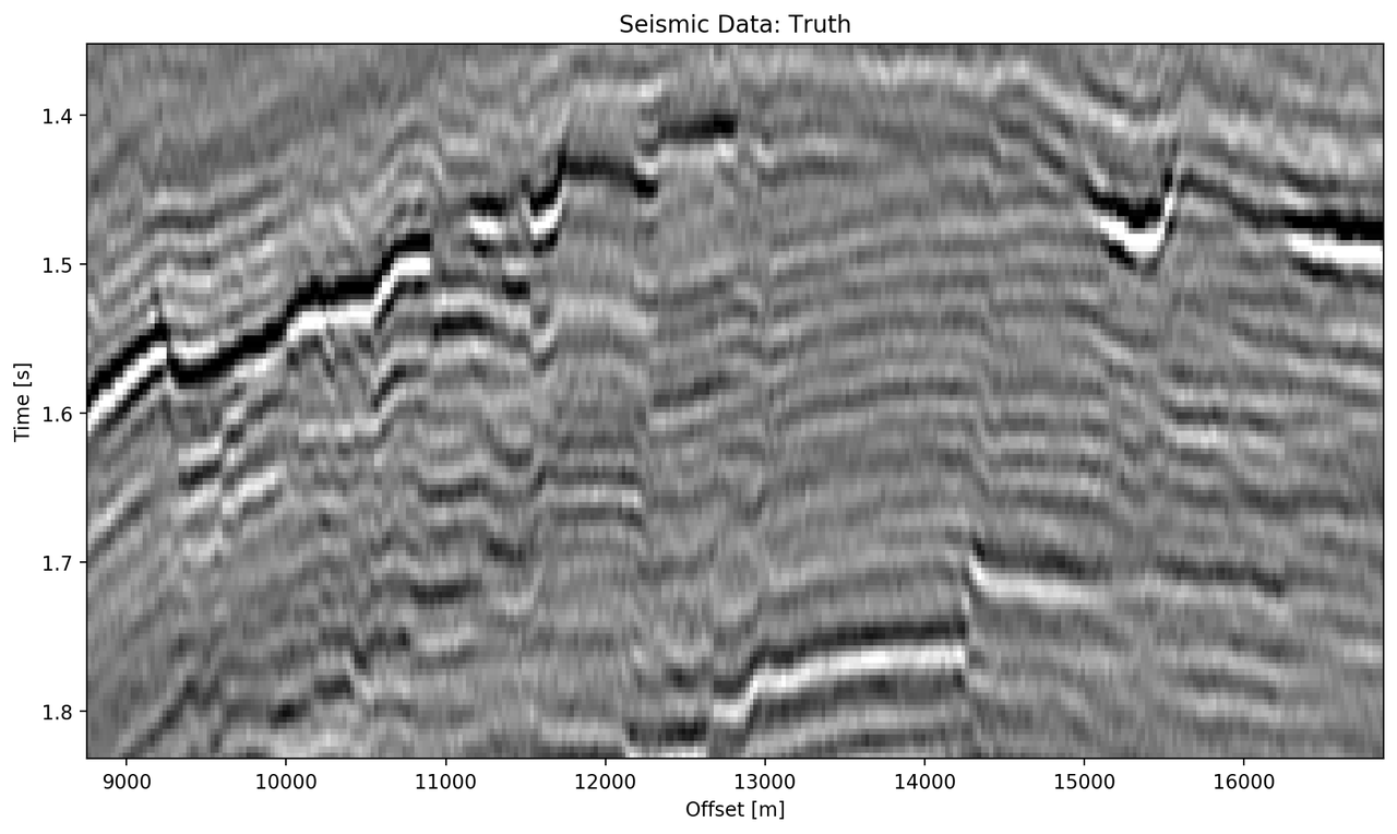
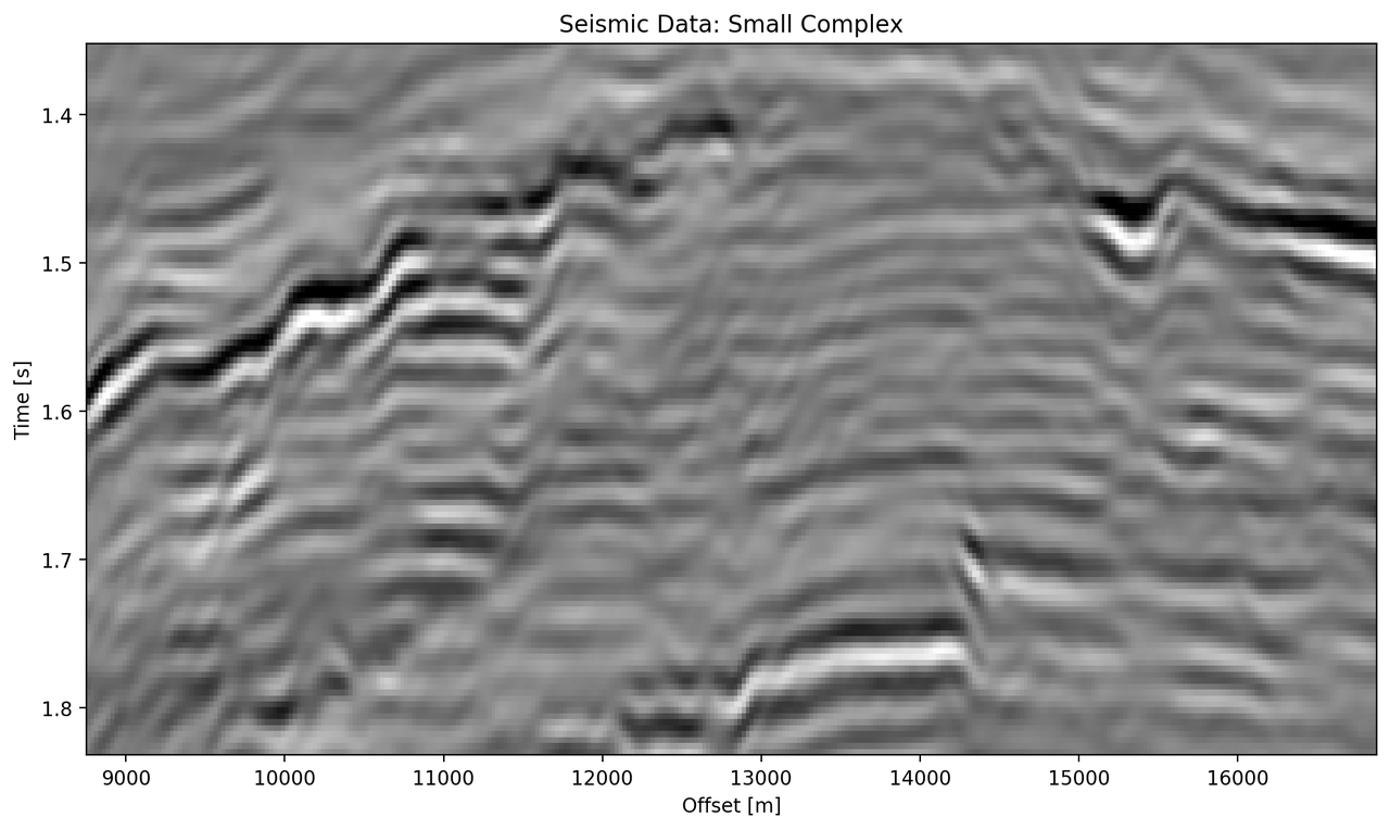
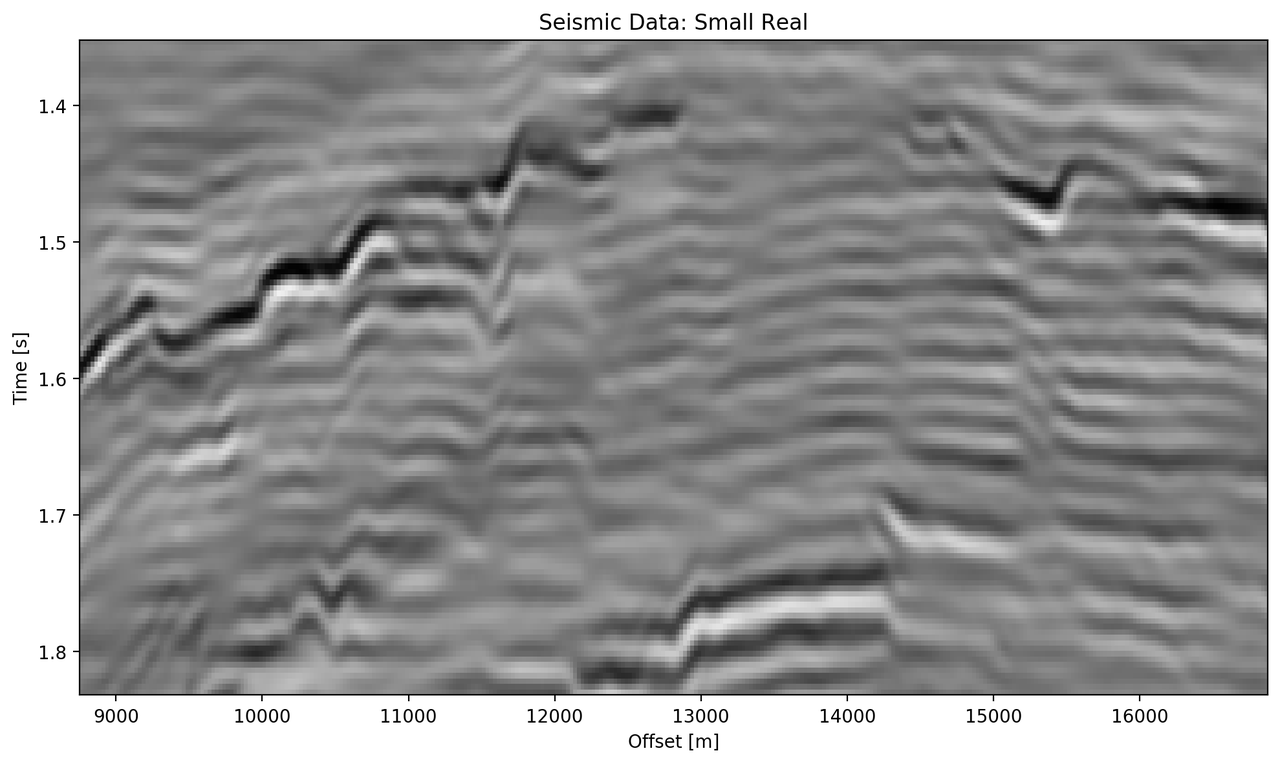
"Bottom" seismic section
The data marked as "bottom" in Figure 5.5 contains a faulted anticline and relatively strong noise levels. The small complex network in Figure 5.9 (d) reconstructs a denoised image with good reconstruction of the visible discontinuities. Some leakage of the reflector starting at 1.5 s across discontinuities is visible. The real small network in Figure 5.9(c) reconstructs a strongly smoothed image, with some ringing below the main reflector, which is not visible in the other reconstructions. The dipping reflector at an offset of 16000 m is well reconstructed, however, it seems like the reconstruction introduced ringing noise over the vertical image. The large real-valued network in Figure 5.9 (e) performs best quantitatively (cf. Table 5.3). The complex-valued large network in Figure 5.9 (d) does a fairly good job at reconstructing the image, similar to the large real-valued network. However, the amplitude reconstruction of high-amplitude events particularly in the main reflector around 1.5 s is showing.
|
|
|
|

|
|
Figure 5.9: Evaluation on Bottom Noise Patch. Data is normalized between -1 and 1.
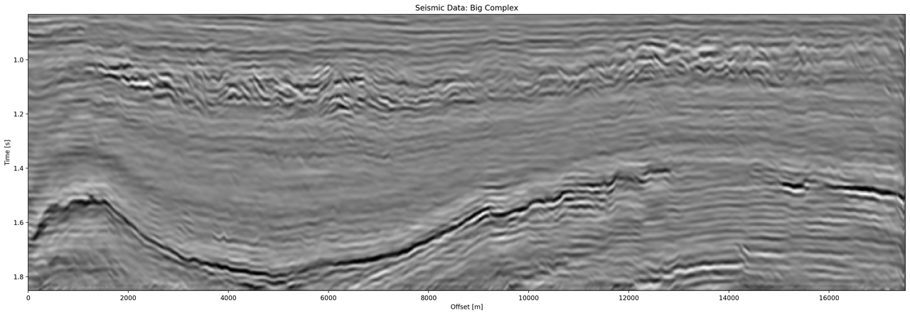
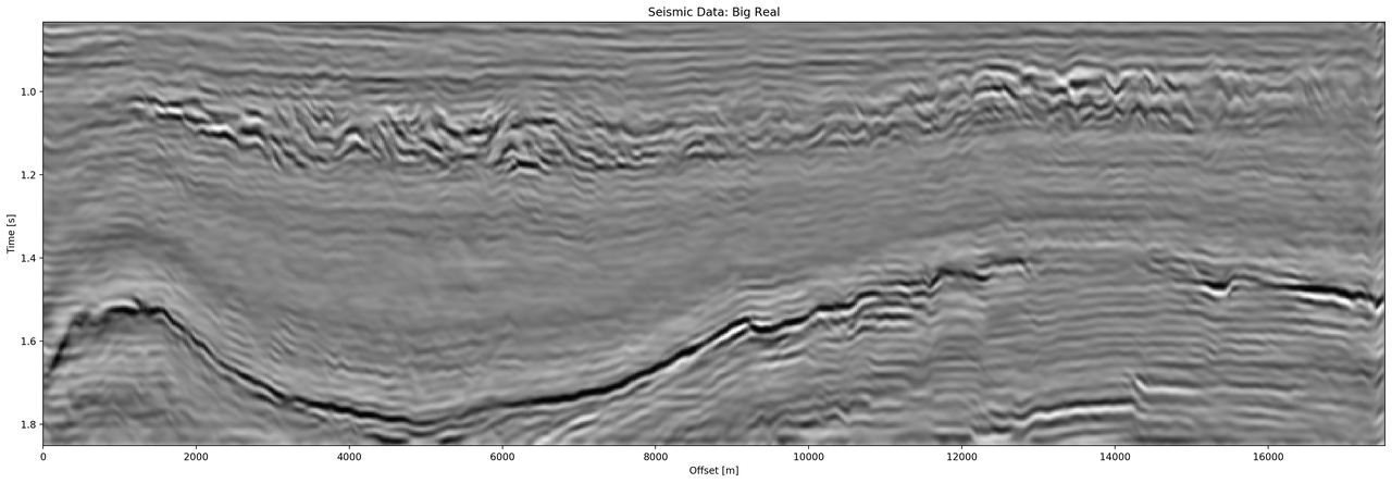
Full seismic test data
It is evident, that the small real-valued network does not match the performance of the smaller complex-valued network, even less so when compared to the large complex-valued network. We therefore compare the large networks on the full seismic data.
|
|
|
Figure 5.10: FK domain of full seismic data.
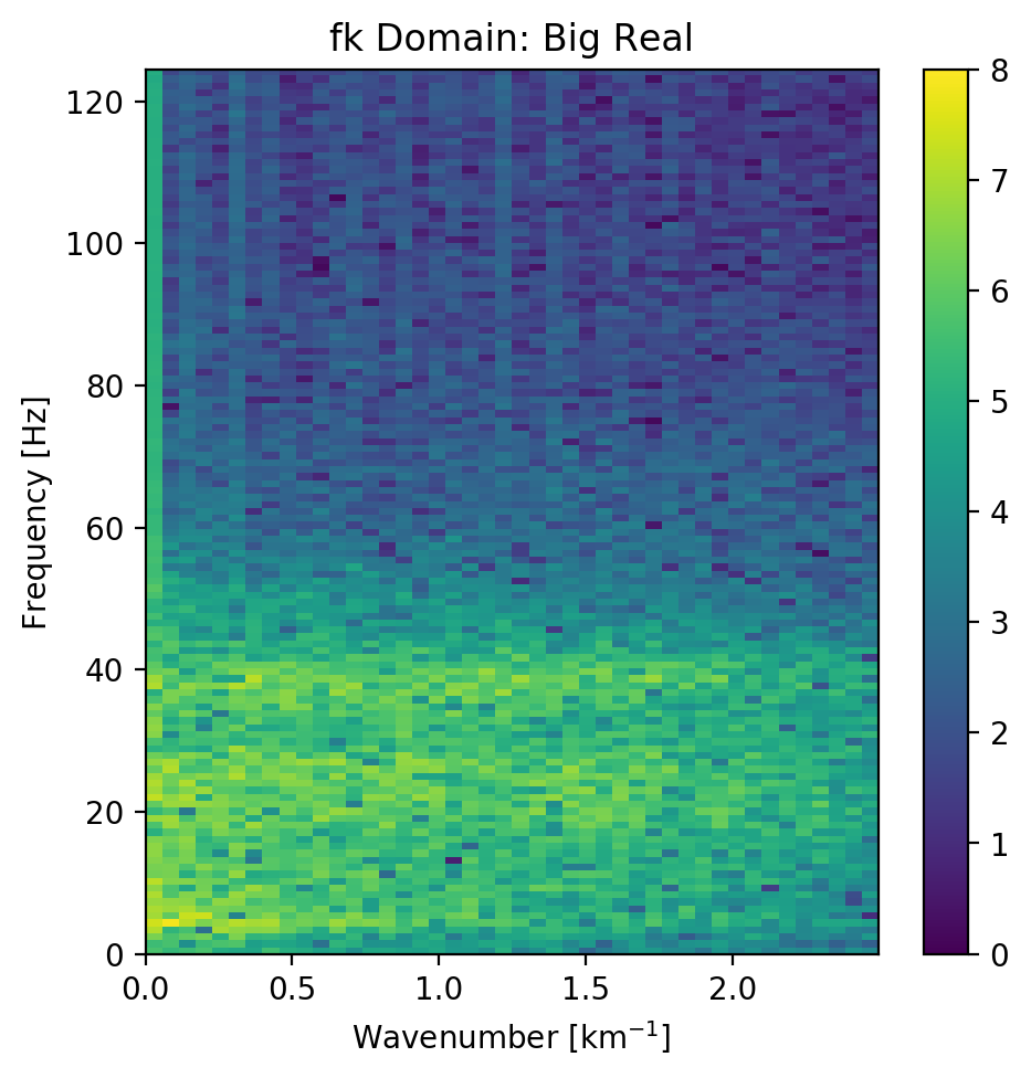
Overall, both networks return a smoothed image. The findings for the strongly faulted sections in the "top" panel hold across the entire faulted area around 1.1 s in Figure 5.11. The complex-valued network does a better job at reconstructing faults and discontinuities. The real-valued network is better at reconstructing high-amplitude regions that appear dimmer in the complex-valued region. The reconstruction of both networks seems adequately close to the ground truth, with differences in the details. Quantitatively, the real-valued network does the better reconstruction in Table 5.3 with an improvement of 2.5 % over the large complex-valued network. The FK domain shows a very similar reduction in noise in the sub 50 Hz band in Figure 5.10. All networks introduce an increase of energy across all frequencies at wave-number \(k=0~km^{-1}\). Additionally, a dimming of the frequencies around \(k=2.5~km^{-1}\) appears in all reconstructions, but is more prominent in the large complex-valued network. The ground truth seismic contains some scattered energy in the high-frequency mid-wavenumber region, visible as "diagonal stripes". These were attenuated in the complex-valued network in Figure 5.10 (b), but are partially present in the real-valued reconstruction in Figure 5.10 (c).
|
|
|
Figure 5.11: Evaluation on full seismic data. Data is normalized between -1 and 1.
Discussion
We evaluated the outputs of the real-valued and complex-valued neural networks. All autoencoder outputs are blurred to different degrees and denoised. The denoising effect of the seismic was most visible in the frequency band below 50 Hz. Additionally, some scattered high-frequency energy was attenuated by the networks.
The largest differences of the outputs in real-valued and complex-valued networks can be observed in discontinuous areas. Particularly, the faulted blocks in the top quarter and in the bottom center of the seismic section show inconsistencies. The real-valued network smooths over discontinuities and steep reflectors. Fault lines are imaged better in the complex-valued network output.
In seismic data processing, including phase information stabilizes discontinuities and disambiguates cycle-skipping in horizons. This could be observed in the network performance and reconstruction. The increase in performance of the real-valued networks was significant (7.0 % RMS), while the complex-valued networks already had an acceptable performance on the smaller network architecture (2.6 % RMS). We provide the complex-valued networks with a bias towards learning phase information, by providing the Hilbert transformed analytical trace, while the real-valued network needs to learn this information implicitly from the data itself. Considering, that during the training, the complex network evaluates both the real-valued seismic, which we primarily care about in addition to the complex-valued component, we can see how the losses in Figure 5.4 differ from the real-valued networks.
The largest network with 790,945 trainable parameters quantitatively performed the best on the reconstruction of the data. However, analysis of the reconstructed seismic shows, that while the high-amplitude regions are reconstructed to higher fidelity, discontinuous sections may be smeared by the real-valued network. The real-valued network that was matched to contain as many filters for the real-valued component of the seismic as the large complex-valued network, did not perform well. Furthermore, the smaller complex-valued network with 100,226 parameters that contains as many filter maps as the real-valued network in total, and half the trainable parameters, outperformed the smaller real-valued network across all test cases.
Conclusion
The inclusion of phase-information leads to a better representation of seismic data in convolutional neural networks. Complex-valued networks perform consistently, where real-valued networks have to learn phase-representations through implicit correlation, which requires larger networks. We show that complex trace information in deep neural networks improves the imaging of discontinuities as well as steep reflectors, particularly in chaotic seismic textures that are smoothed by real-valued neural networks of the same size and level of compression.
We show that convolutional neural networks can perform lossy compression on seismic data, where the reconstruction error is dependent on both network architecture and implementation details, like providing explicit phase information. During this compression, noise and scattered energy get attenuated. The real-valued network is prone to introduce steeply dipping artifacts in the reconstruction and is matched by complex-valued networks half the size with twice the amount of compression. This is particularly interesting in the light of the complex complement of the data being derived from the real-valued data through a Hilbert transform, which should have been possible to approximate by a neural network.
The stabilization of the reconstruction can be useful in other seismic applications. While automatic seismic interpretation may benefit from the inclusion of information on discontinuities, we see the main application to be lossy seismic compression. The open source tool developed to make this research possible, enables further research and development of complex-valued solutions to non-stationary physics problems that benefit from explicit phase information.
This research also shows that a change as small as 2.5 % in RMS can change the reconstruction from being acceptable to very smeared to a geoscientist. This touches on the fact that better metrics to evaluate computer vision tasks in geoscience are necessary. Additionally, these tasks have to be noise-robust and, while amplitude-preserving, be robust against outliers. Moreover, more research in the frequency dimming of bands in the network reconstruction is necessary.
Overall, the computational memory footprint of the complex convolution is higher than real-valued convolutional neural networks comparing singular convolutional operations. A significant increase in depth and width of networks to obtain an acceptable result in real-valued neural network to implicitly learn the phase information is necessary. The complex-valued networks an 8th of the size already performs well, suggesting that domains where a significant part pf the information is in the phase of signals, could benefit from applying complex convolutional networks.
Acknowledgments
We thank Andrew Ferlitsch for his valuable insights. The research leading to these results has received funding from the Danish Hydrocarbon Research and Technology Centre under the Advanced Water Flooding program. We thank DTU Compute for access to the GPU Cluster.
Contributions of this Study
This chapter and Jesper Sören Dramsch, Lüthje, and Christensen (2019) investigate the application of complex trace analysis to convolutional neural networks. It uses lossy compression to measure the reconstruction error and therefore, the informational content in complex-valued neural networks. We were able to show that networks containing phase information in the complex complement of data reduce the error as compared to real-valued networks. Moreover, the code to reproduce the findings in this paper (Jesper Sören Dramsch 2019b), as well as, a standalone Python library for complex-valued convolutional neural networks in tensorflow has been made available as foss (Jesper Sören Dramsch and Contributors 2019).