End-to-End convolutional neural network training

End-to-End convolutional neural network training
~~~~~~~~~~~~~~~~~~~~~~~

The training of the Waldeland convolutional neural network is trained end-to-end. The optimizer for the Waldeland convolutional neural network is the Adam optimizer (Diederik P. Kingma and Ba 2014) with a learning rate of \(0.001\), the decay of first-order moments of \(\beta_1=0.9\), and second-order moments of \(\beta_2=0.999\).

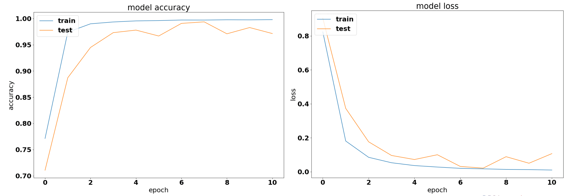
Accuracy and Categorical Cross Entropy for Waldeland convolutional neural network

13.2 shows the training loss of end-to-end training. The accuracy shows that the network very quickly reaches 100% accuracy on the training data while performing close to perfect on the test set. The training is stopped after ten epochs. The loss shows that the model starts overfitting at epoch 7. A dataset with more diverse labels and samples would improve this situation.

Fine-Tuning Pre-Trained Networks

Pre-trained networks were trained on a dataset and made available by the researchers and companies, including weights and biases. These are often trained on large corpuses of data. In computer vision, classically pre-trained networks were trained on ImageNet, CIFAR, and PASCAL-VOC. The sota networks are pre-trained on up to a billion images with 17,000 labels and subsequently fine-tuned on the ImageNet-1K dataset (Mahajan et al. 2018). This strategy is applied across deep learning, including computational linguistics with 175 billion parameters pre-trained on 0.499 trillion words in GPT-3 (Brown et al. 2020). The pre-trained networks in this chapter were trained on the ImageNet corpus and transferred to the MaleNov seismic dataset (Ildstad and Bormann 2017).

The VGG-16 and ResNet-52 are finetuned using sgd with Nesterov momentum. The learning rate for the sgd is set to \(0.0001\), with a momentum of \(0.9\). Additionally, a learning rate schedule is implemented that updates the learning rate (lr) according to \(lr(t) = 0.0001 \cdot \left( 1 + 10^{-6} \cdot t \right)^{-1}\).

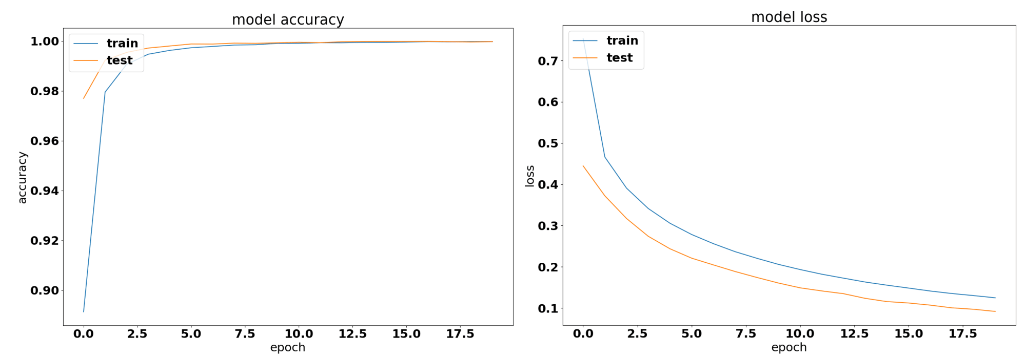
Accuracy and Categorical Cross Entropy for VGG16 convolutional neural network

The VGG-16 network quickly converges to 100% accuracy, the loss, however smoothly converges towards a cross-entropy of \(0.1\). The network does not show signs of overfitting and trains the full 20 epochs. With the available hardware at the time of writing the paper and the good results despite possibly increasing the convergence.

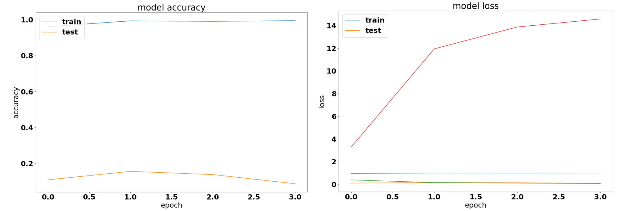
Accuracy and Categorical Cross Entropy for ResNet52 convolutional neural network

The ResNet-52 network immediately reports a training accuracy of close to 100% while the test data report 11% accuracy, which is a performance equivalent to random chance on this dataset containing nine classes. The loss in 13.4 shows the same problem of a massively overfit network. For this reason, the network predictions were not displayed in the paper in this chapter.

Introduction

Seismic interpretation is often dependent on the interpreters experience and knowledge. While deep learning cannot replace expert knowledge, we explore the accuracy of convolutional networks in interpreting seismic data to support human interpretation.

In the 1950s neural networks started as a simple direct connection of several nodes in an input layer to several nodes in an output layer (Widrow and Lehr 1990). In geophysics this puts us to the introduction of seismic trace stacking (Öz Yilmaz 2001). In 1989 the first idea of a convolutional neural network was born (Lecun 1989) and back-propagation was formalized as an error-propagation mechanism (D. E. Rumelhart, Hinton, and Williams 1988). In 2012 the paper (Krizhevsky, Sutskever, and Hinton 2012a) propelled the field of deep learning forward implementing essential components, namely GPU training, ReLu activation functions (Dahl, Sainath, and Hinton 2013) and dropout (Srivastava et al. 2014). They outperformed previous models in the ImageNet challenge (J. Deng et al. 2009) by almost halving the prediction error. Anders Waldeland and Solberg (2016) showed that neural networks can be used to classify salt diapirs in 3D seismic data. Rutherford Ildstad and Bormann (2017) generalized this work to nD and beyond two classes of salt and "else".

The task of automatic seismic interpretation can be equated to dense object detection (T.-Y. Lin et al. 2017) or semantic segmentation. These tasks are currently best solved by Mask R-CNN architectures (Long, Shelhamer, and Darrell 2015). Statoil has used U-Nets for automatic seismic interpretation. Yet, classification networks can be used for semantic segmentation, but are significantly slower. The benefit is a testable example of generalization of pre-trained networks form photographic data to seismic images. As well as, a testable framework for choosing hyper-parameters for neural networks on seismic data.

Deep learning relies heavily on vast amounts of labeled data to train on initially. However, the features learned from these networks can often be transferred to adjacent problem spaces (Baxter 1998). Often these transfer learning tasks are tested on photographs rather than seismic or medical imaging tasks. The aim of this study is to evaluate state-of-the-art pre-trained networks in the task of automatic seismic interpretation. We compare three convolutional neural networks of increasing complexity in the task of supervised automatic seismic interpretation. We evaluate these tasks qualitatively and quantitatively.

Methods

The neural networks in this study learn supervised. The features were published alongside the open source framework MalenoV and describe nine seismic facies in the open F3 data set. The classes describe steep dipping reflectors, salt intrusions, low coherency regions, low amplitude dipping reflectors, high amplitude regions continuous high amplitude regions and grizzly amplitude patterns presented in figure 13.7. Additionally, a catch-all “else” region are picked. In this approach we chose Keras (Chollet and others 2015a) with a Tensorflow (Abadi et al. 2015a) backend on a K5200 GPU at DHRTC. Keras is a high level abstraction of tensor arithmetics. Tensorflow is an open source numerical computation library on static graphs. We train 2D convolutional neural networks (CNN) of varying depth on seismic slices to propagate single slice interpretations to a volume. CNNs are highly flexible models for computer vision tasks.

Network one depicted in figure 13.5 was developed by (Anders Waldeland and Solberg 2016) to identify salt bodies in 3D seismic data. Three layers are fully connected for classification. The network uses a kernel of 5 by 5 pixels for convolution and a stride of 2 for down-sampling. We use the Adam optimizer and cross-categorical entropy as a loss function. The Adam optimizer is an extension to stochastic gradient descent (SGD) that implements adaptive learning rates and bias correction (Ruder 2016). We add dropout and batch normalization to the network. These methods improve regularization and prevent overfitting. Furthermore, we use early-stopping to prevent overfitting the model by over-training. We chose two metrics to monitor in the training and validation sets, namely mean absolute error and accuracy. The Waldeland convolutional neural network is relatively shallow compared to modern deep learning networks with 95,735 parameters to optimize for.

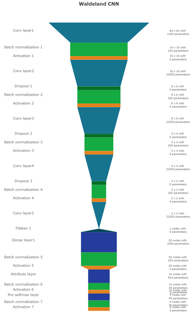
Waldeland convolutional neural network architecture. Input at the Top. Softmax Classification Layer on bottom. Width of objects shows log of spatial extent of layer. Height shows log of complexity of layer. The layers are color coded to show similar purpose.

Network two is the VGG16 network (Simonyan and Zisserman 2014b) by the Visual Geometry Group. It contains 16 layers and 1,524,2605 parameters. 13 of these layers ore convolutional layers with a 3x3 kernel. Convolutional blocks are interspersed with max-pooling layers for down-sampling. The last three layers are fully connected layers for classification. The VGG16 architecture was proposed for the ImageNet challenge in 2013. It is widely used for it’s simplicity in teaching and it’s generalizability in transfer learning tasks.

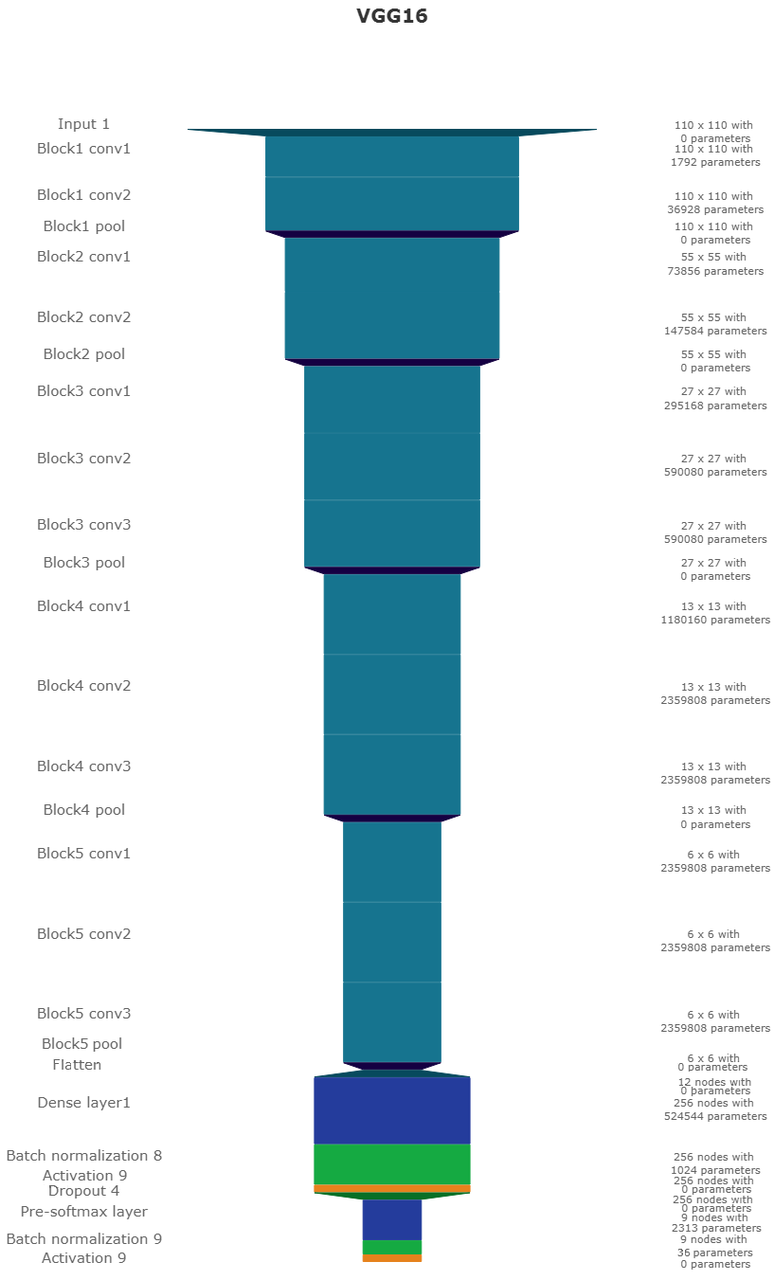
VGG16 architecture. Same visualization as figure 13.5

Network three is the ResNet50 architecture by Microsoft. The network consists of 50 layers with 2,361,6569 parameters. It implements a recent development, called residual blocks. These residual blocks add a skip- or identity-connection around a stack of 1x1, 3x3, 1x1 convolutional layers (K. He et al. 2016). The 1x1 are identity convolutions, used for down- and subsequent up-sampling to decrease the computational cost of very deep convolutional neural networks. The convolutional layers are followed by one fully connected layer for classification.

All networks use rectified linear units (ReLu) as neural activation. The last layer uses Softmax as activation to output a probability for each class. Training both VGG16 and the ResNet50 end to end would be very expensive. These models have been trained on big labeled data that are not available in geoscience. However, transfer learning enables us to use pre-trained networks on very different tasks. In transfer learning, we use the learned weights of the networks and replace the fully connected layers. These untrained layers are specific to our task and have to be fine-tuned to the data. This process is very fast and requires little data. We fine-tune an entire network on one sparsely interpreted 2D seismic slice. For the fine-tuning process, we replace the Adam optimizer by a classic SGD optimizer with lower learning rate, very low weight decay and Nesterov momentum. We still use early-stopping on validation loss and cross-categorical entropy.

We added the same fully connected layer architecture to VGG16 and ResNet50 that Waldeland added to their architecture. Therefore, we test if pre-trained convolution kernels are fit to recognize texture features in seismic data. We set up a validation set to quantify the accuracy of our networks on previously unseen data. Additionally, we set up a prediction pipeline to populate each one 2D inline and crossline of the seismic data to qualitatively visualize the prediction capability of the networks. The labels for the supervised interpretation are taken from the MalenoV interpretation by ConocoPhillips, shown in figure 13.7.

.. table:: Training and Test scores on Networks. Test scores are prediction results on a labeled hold-out data set. Mismatch of test and training scores indicates over-fitting.

   ============= ======== ====== ===== ======
   Network       Run      Loss   MAE   Acc
   ============= ======== ====== ===== ======
   Waldeland convolutional neural network Training 0.001  0.000 100.0%
                 Test     0.003  0.000 99.9%
   VGG16         Training 0.010  0.005 99.8%
                 Test     0.127  0.026 100.0%
   ResNet50      Training 0.011  0.001 100.0%
                 Test     14.166 0.195 12.1%

   ============= ======== ====== ===== ======

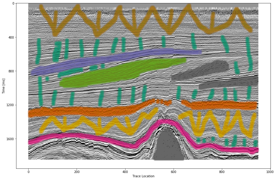
Labeled data set on one 2D inline slice. Color interpretation: Low coherency (brown), Steep dipping reflectors (gray), low amplitude dipping reflectors (grass green), continuous high amplitude regions (blue), grizzly (orange), low amplitude (yellow), high amplitude (magenta), salt intrusions (gray), else (turquoise).

Results

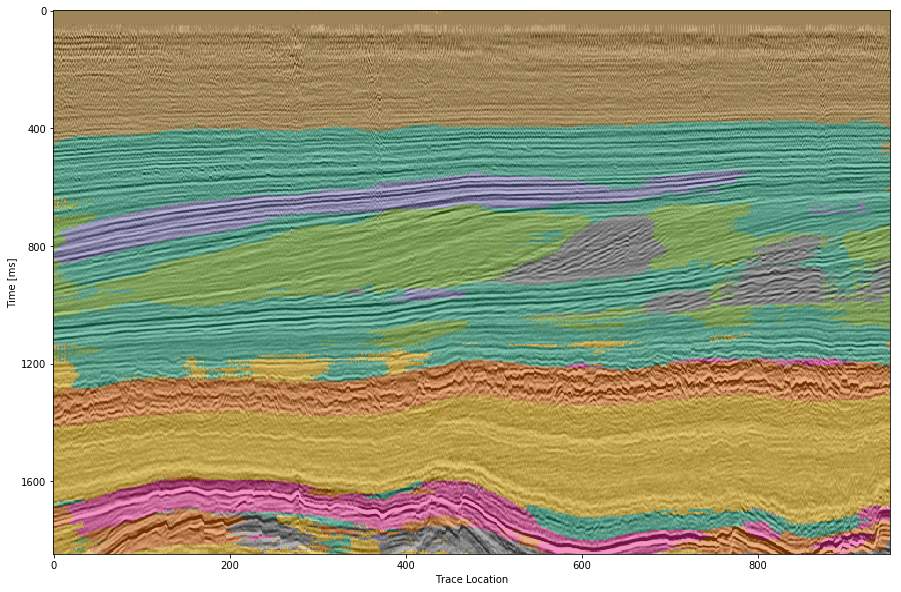
We use the open Dutch F3 data set to calibrate our predictions. Crossline 339 has been interpreted by ConocoPhillips and made available freely. We show results of crossline slice 500. We have used the same plotting parameters for both either results, both have been generated programatically, without human intervention. Figure [transfer:fig:predi] shows the prediction of the Waldeland convolutional neural network at every location of the 2D slice based on a 65 x 65 patch of the data. Border patches were zero padded. We see clear patches for the low coherency region in brown. The low amplitude dipping (grass green) region has been reproduced well, however some regions at \(t\approx1080~\text{ms}\) have been marked incorrectly, where two seismic packages meet. This faulty region also contains patches that were interpreted as low amplitude region (yellow). While this may be a low amplitude region, we expect the packages to be largely continuous, which leaves this interpretation as questionable at best. The gray area was reproduced well, however it was marked as salt body in the original manuscript, this would be incorrect here. We see the grizzly amplitude pattern (orange) and the low amplitude (yellow) regions are well-defined and separated. The underlying package of high amplitudes has been identified will. However, between location 600 - 800 the top part was marked as "else" (turquoise), which undesirable but correct, judging from the texture. Here, retraining would be possible by feeding this relabeled region to the network. Below this region, the networks predictions become erratic. The classification is blocky between grizzly and salt with "else" interspersed. However, the edges will often give problems due to the padding. Around location 800 high amplitudes (orange) have been mislabeled as grizzly amplitudes.

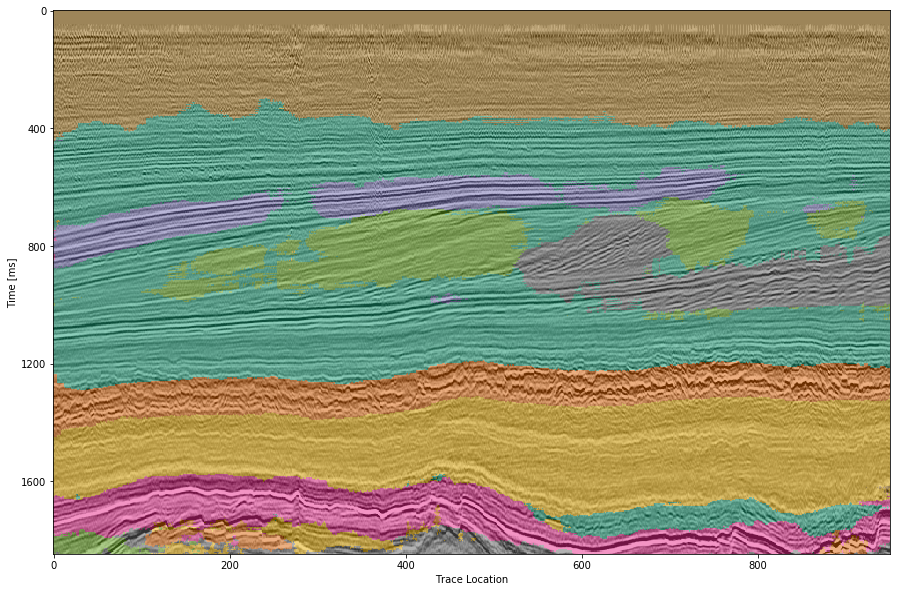
The VGG16 network classification is shown in figure [transfer:fig:vggpredi]. The network performs similar to the Waldeland convolutional neural network in figure [transfer:fig:predi], however some key differences will be pointed out. The separation of low coherency and the "else" region around \(t\approx400~\text{ms}\) is less defined and, therefore, worse. The coherency of low amplitude dipping (grass green) and high amplitude continuous (blue) is worse in the region around location 280, \(t\approx800~\text{ms}\). This might be due to higher sensitivity to declines in seismic quality. Below \(t\approx1000~\text{ms}\) the "else" region is free from differing patches, in contrast, the Waldeland convolutional neural network interspersed two other classes in this region. VGG16 also classifies some "else" regions in the high amplitude (magenta) region between location 600-800. The area around location 200 below the high amplitude (magenta) region is also blocky, although less so. The misclassification of the bottom high amplitude (magenta) region as grizzly (orange) is less pronounced in the VGG16 interpretation. It is present toward the bottom left corner.

The results of the ResNet50 are not shown. The network classifies all seismic facies as "else". This indicates that the network is overfitting the data. This is supported by the numeric results presented in table 13.1. The network training error indicates a perfect fit to the data, whereas the test score is unseen data with labels to evaluate the performance of networks on unseen data. While both the Waldeland convolutional neural network and VGG16 perform well, the ResNet50 performs very poorly.

Conclusion

Convolutional neural networks show good results for propagating interpretations through seismic cubes. The pre-trained VGG16 convolutional neural network has shown very good results in adapting to seismic texture identification. Transfer learning was fast and the results are similar to the shallower Waldeland convolutional neural network. Both networks have trade-offs in the misclassification and can be improved upon.

The ResNet50 was shown to be ineffective on transfer learning seismic data with pre-trained weights. This is in accordance with results from other attempts at transfer learning. The ResNet filters are more specific to photography and transfer poorly to other data sources, where the VGG learned features prove to be more general to computer vision tasks. More complicated architectures may perform well, trained directly with the according data, but they learn specific features fit for the problem space that do not transfer well.

Acknowledgments

The authors would like to thank the DHRTC and DUC for their continued support. We thank Colin MacBeth, Peter Bormann, Sebastian Tølbøll Glavind, Lukas Mosser and the "Software Underground" community for great discussion and support with MalenoV and ConocoPhillips for making the data and software freely available. We also thank Agile Scientific for great tutorials at the intersection of Python and geoscience. We thank dgb for providing the F3 data set.