Unsupervised Geological Image Segmentation
Dramsch, J. S., Amour, F., & Lüthje, M. (2018, November). Gaussian Mixture Models for Robust Unsupervised Scanning-Electron Microscopy Image Segmentation of North Sea Chalk. In First EAGE/PESGB Workshop Machine Learning. |
|||
Github: https://github.com/JesperDramsch/backscatter-sem-segmentation |
|||

Analysis of chalk samples can be done by bsem. The resulting images contain black-white images of the sample that can be measured and analysed. The back-scatter measurements add information regarding the chemical composition from the back-scattered energy from the electron beam. Research into the porosity and sedimentology of the chalk reservoirs conducted using electron microscopes. Identifying the grain size and orientation of the oolites is usually a manual work-intensive task, ideal for computer vision tasks, considering the good contrast of light-grey to white oolites and the black background. [fig:bsem] shows a chalk sample from the analysis. The chalk grains are of varying size, with inter- and intra-grain porosity. The intra-grain porosity is best seen in the grain located at \((1000, 200)\) in [fig:bsem]. bsem data is noisy, which can distort the image. Additionally, grain boundaries tend to be jagged, which is aggravated by the noise.
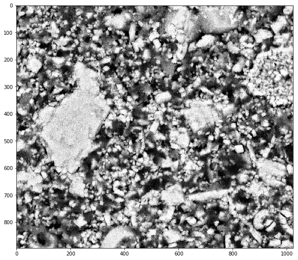
Backscatter SEM image of chalk data
Unsupervised Image Segmentation
Labelled training data was not available to apply convolutional neural networks to this problem. Instead of hand-labelling the data, unsupervised clustering was appropriate to find the optimal boundary of the grains from the background. gmms learned a two-fold representation that separated the background well from the rock. Clustering the pixel intensity into two clusters with the gmm and classical histogram boundary are displayed in 12.1. These boundaries do not coincide, and while they are close, the two-pixel difference changes the prediction significantly.
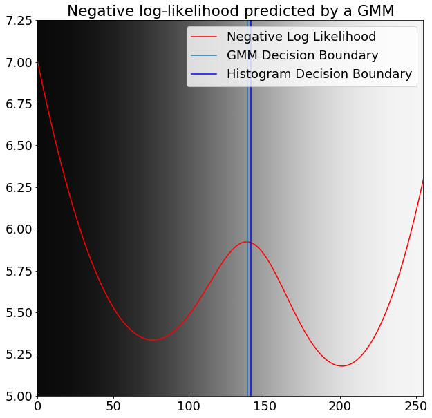
Greyscale values overlaid with negative log likelihood predicted by gmm (red) with decision boundaries from gmm (green) and histogram decision boundary (blue).
Gaussian Mixture Models
In detail, the gmm can model normally distributed sub-populations that constitute a larger population. The Gaussian distributions are usually estimated by using the maximum likelihood method. Because differentiating the log-likelihood is computationally infeasible, commonly, the expectation maximisation (EM) is utilised to approximate the maximum log-likelihood. EM is an iterative approach that calculates the expectation of a sample to be part of a component and maximisation, which updates the model parameters.
We define \({x} = (x_1, x_2, ..., x_n)\) as the data points with \(n\) independent observations. Then \({z} = (z_1, z_2, ..., z_n)\) is the latent vector and \(X_i | (Z_i = k) \propto \mathcal{N}_d(\mu_1, \Sigma_1)\) for \(k\) compononents and a \(d\)-dimensional Gaussian. Then the distribution
where \(\phi_i\) are the model weights and normalize to
The Expectation step calculates the membership probabilities for all samples \(i\) and components \(k\):
then the estimated \(\hat{\gamma}_{ik}\) describes the probability that a sample \(x_i\) is generated by the \(k\)-th component \(C_k\), leading to the conditional probability \(\hat{\gamma}_{ik} = p(C_k|x_i, \hat{\phi},\hat{\mu},\hat{\sigma})\).
The Maximization step then updates the parameter set \((\hat{\phi}, \hat{\mu}, \hat{\sigma})\) for all k:
The parameters are initialized by a naive strategy, so that all samples in \({x}\) get randomly assigned to a component and the weights are uniformly distributed as \(\phi_1, \phi_2, ..., \phi_K = \frac{1}{K}\). The iteration is stopped when the model converges, that is the expectation of subsequent steps changes less then a pre-set \(\epsilon\).
Morphological Filtering
This single-valued intensity value causes the boundary to be non-smooth around the grains. Therefore morphological filtering was applied to smooth out the boundaries programmatically. Smooth boundaries are essential for chalk grains, as the perimeter of the oolites can be used to calculate the specific surface of chalk. The optimal boundary of chalk grains could then be used to generate training data for more sophisticated machine learning systems.
Mathematical morphology is the theory of analysing geometrical structures. Morphological filtering implements multiple shape-based filters that perform non-linear transformations. In this case, we apply morphological dilation and morphological erosion. Morphological erosion set the central pixel to the minimum of a neighbourhood. More formally \(A\) is a binary image and \(B\) is a structuring element on the Euclidean space \(E\), e.g. a \(3\times3\) square, or a disk with defined radius, then \(A \ominus B = \{z\in E | B_{z} \subseteq A\}\), where \(B_z\) is the translation of \(B\) by the vector \(z\). More concisely morphological erosion is:
The morphological dilation, in turn, sets a central pixel to the maximum of the neighbourhood of pixels in an image. Then
These operations can then be combined to perform morphological opening, which is commonly used to "clean up" edges in binary images. Morphological closing can be written as
Repeating erosion and dilation alternatingly smoothes out the boundary we obtain from gmm.
Workshop Paper: Gaussian Mixture Models For Robust Unsupervised Scanning-Electron Microscopy Image Segmentation Of North Sea Chalk
Introduction
In the oil and gas industry, assessment and prediction of the hydrocarbon reserves and flow properties throughout a chalk reservoir lifetime relies, among others, on conventional and special core analysis (CCAL and SCAL) and computed tomography (CT) imaging in order to characterise the petrophysical properties and 3-D pore network geometry of chalk.
The latter laboratory experiments are technically challenging, costly, and time-consuming and require a large amount of core material. Various image analysis techniques, studying the 2-D distribution of grains, pores, and pore throats on thin-sections, have been extensively tested over more than 50yrs for workflow optimization.
Nevertheless, such techniques have not yet been integrated by reservoir engineers and geoscientists as a routine task during reservoir characterization, especially, due to a limited number of samples tested or a spatially-restricted study area that do not allow the results to be statistically representative of the chalk heterogeneity across a reservoir and between oil and gas fields.
Back-scattered electron microscopy (BSEM) analysis historically has been very manual work. Separating grains from the background, measuring perimeter and area of the grains. Recently, publications showed automatic segmentation of BSEM images using computational methods. The present study represents a robust method in the application of machine learning on thin-section images collected by BSEM. This cheap and relatively rapid technique allows to quickly analyse a large number of pictures that do not need to be manually labeled.
Method
SEM Analysis as Image Segmentation
Scanning Electron Microscopy (SEM) is an imaging method that allows the visualisation of the grains and pores of chalk deposits (Figure 12.2). Grayscale images of the rock fabric can be collected at various scales of observation, from the micro-scale, typically single pore and grain, to few tens of microns where the network of pores can be studied, to the millimetres-scale. This provides a complete insight of the heterogeneity of each sample. Nanotube SEM and many applications separate very well the grains from the background in the SEM images. Therefore, these images can be segmented by histogram methods. Carbonates and specifically chalk vary on grayscale, and grains are not illuminated homogeneously. However, image segmentation has made many improvements in recent years, which extends the toolkit beyond histogram segmentation.
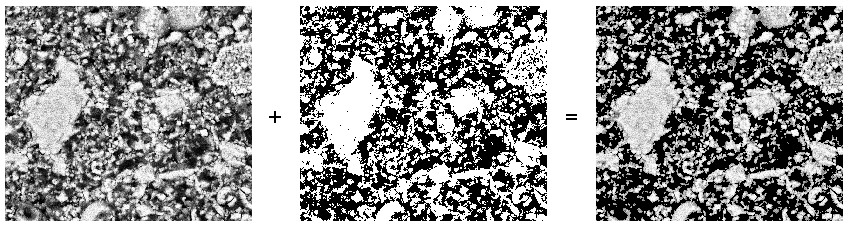
Original SEM image, binary mask obtained by GMM, and resulting grain image.
Modern Neural Networks (NN) can segment images exceptionally well (Ronneberger, Fischer, and Brox 2015b). Modarres et al. (2017) investigated the application of neural networks to SEM images. However, as with most applications in Geoscience and supervised learning, we would have to label a significant amount of images by hand to assure quality or automatically with subpar methods to train the network adequately. This defeats the point for this application, therefore, this study investigates unsupervised methods, which will be assessed in order to select the one that performs the best across all scales of observation. Several BSEM images of the rock fabric at the same scale are also collected to validate the results.
Gaussian Mixture Model (GMM) learns a number of joint distributions approximated by Gaussians in the search space (Lindsay 1995). The number of Gaussians has to be specified, similar to many clustering methods, like k-means. In this application, we aim at segmenting the background from the chalk, which lends itself to specify two Gaussian distributions as learning parameter to obtain a binary mask, presented in Figure 12.2.
Morphological Filtering
Filtered segmentation of BSEM
We apply morphological filtering to clean up the segmentation (Serra and Vincent 1992). Due to the noisy images of BSEM, the edges of grains appear fuzzy. For the automatic analysis of the perimeter for instance, seen in Figure 12.3.
Subsequently, we can programmatically analyse the result using scikit-learn and scikit-image (F. Pedregosa et al. 2011). This provides area, perimeter and rotation of grains in the image among other geometrical factors of the grains. These can be very valuable in digital rock physics and pore analysis.
Conclusions
We present an effective segmentation method for BSEM image data. Gaussian Mixture Models learn a good representation of the grayscale data and morphological filtering further improves the results.
Acknowledgements
The research leading to these results has received funding from the Danish Hydrocarbon Research and Technology Centre under the Advanced Water Flooding program.
Computational Granulometry
Identifying the grains in an bsem image enables us to perform computational granulometry on the images. The segmented images can be analysed with standard image processing algorithms that can return standard measures such as perimeter, area, and eccentricity of grains. Moreover, depending on the preparation of the chalk sample, the angle of orientation can be extracted for each grain.
[fig:grainsizes] shows the distribution of grain sizes over the image. The data shows an even distribution toward smaller chalk grains, with three very large samples, that can be clearly identified in 12.4. [fig:uncircular] shows the shape distribution of the grains, which is distributed toward less circular grains due to compaction. Nevertheless, there are two strong spikes toward circular grains which is in accordance with our expectation for chalk oolites.
Moreover, this analysis enables us to calculate the approximate porosity from the image. The porosity calculated is 44.25%. The measured porosity of the chalk sample is 42%, which is close for a 2D image of the 3D pore space.
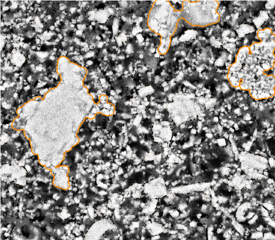
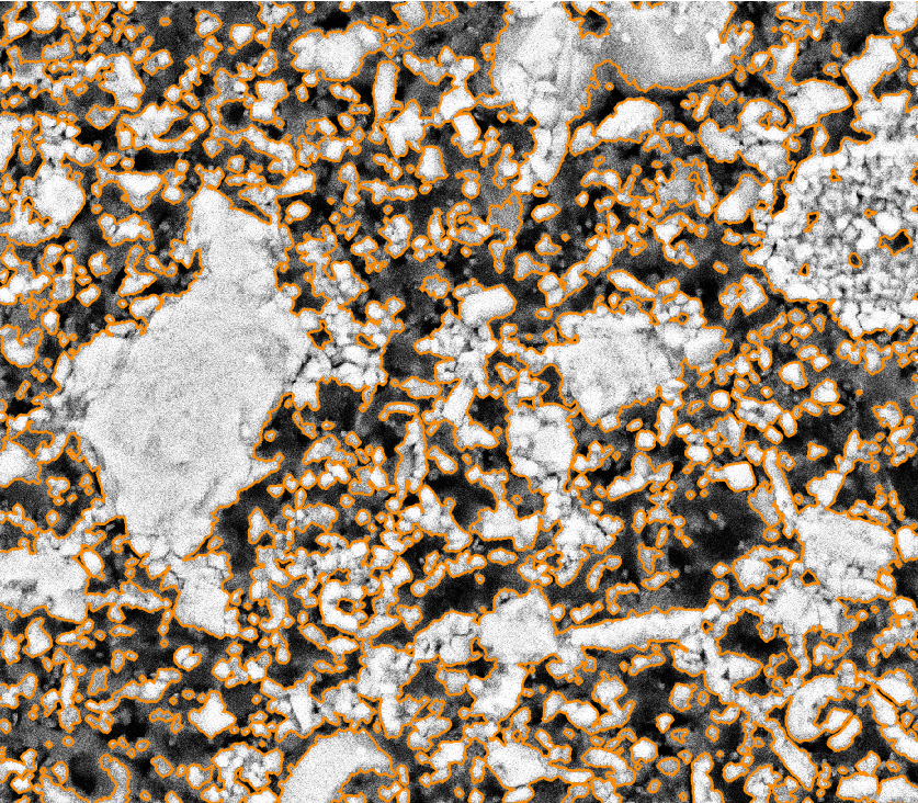
bsem data with three large chalk grains outlined from the gmm process (orange). The image shows mostly brecciated chalk grains with some interspersed circular oolites.
Contributions of this Study
This study introduced unsupervised gmm clustering for chalk grain bsem image segmentation. Overall, the method shows a very good separation of the grains from the background in the image. The method performs well on images with varying lightness, due to the unsupervised nature of the gmm algorithm. This model, however, benefits from the contrast between the light chalk grains and the dark background. Nevertheless, it does outperform classical methods, i.e. a histogram-based analysis.
Morphological filtering improves the segmentation of the image. The morphological filtering application is computationally efficient and reliable in removing small scale variations in the data. The morphological opening smoothes the boundaries between the grain and the background and remove small grains and possible noise from the binary labels.
These binary labels enable computational granulometry on the grain data. This data has good accordance with the image data, as well as measured porosity on the rock sample. Finally, this method can be used to generate labels for more complex machine learning models, i.e. convolutional neural networks.
The code of this analysis is published under .