Machine Learning in 4D Seismic Inversion
Dramsch, J. S., Corte, G., Amini, H., MacBeth, C., & Lüthje, M.. (2019). Including Physics in Deep Learning–An example from 4D seismic pressure saturation inversion. arXiv preprint arXiv:1904.02254. |
|||
Github: https://github.com/JesperDramsch/4D-seismic-neural-inversion |
|||

Dramsch, J. S., Corte, G., Amini, H., Lüthje, M., & MacBeth, C.. (2019, April). Deep Learning Application for 4D Pressure Saturation Inversion Compared to Bayesian Inversion on North Sea Data. In Second EAGE Workshop Practical Reservoir Monitoring 2019. |
|||
Github: https://github.com/JesperDramsch/4D-seismic-neural-inversion |
|||
This chapter discusses a neural network application to approximate the pressure-saturation inversion of 4D seismic data. It contains two workshop papers that discuss two different aspects of the construction of the neural network architecture. Traditionally, 4D seismic qi often relies on priors to reduce variance in the face of uncertainty. The inversion problem in this chapter is a pressure-saturation inversion from seismic amplitude difference maps in the Schiehallion field. The first paper presents an ablation study of the components in the architecture. The second paper discusses the neural network result and presents a comparison to a classical Bayesian inversion.
Data
The Schiehallion field is a stacked turbidite reservoir in the UK North Sea, which makes it very heterogeneous and compartmentalized. The T31 sandstone reservoir has the most lateral extent with the thickness ranging from 5 m to 30 m. The small thickness of the reservoir layer results in the entire reservoir being contained in a single trough of a seismic wavelet (\(\approx\frac{1}{2}\lambda\)), which has historically lead to applications using a 2D map view of the data. In order to make the results comparable, we treat the network as a 2D map instead of a 3D problem.
The data available consists of simulation and field data with several years of collected seismic data. The baseline acquisition is from 1996 with additional time steps acquired in 1999, 2000, 2002, 2004, 2006, 2008, and 2010. There are simulation results and measured amplitude difference maps. The simulated seismic data is based on pore volumes from previous pore volume inversions, pressure changes and saturation changes for water and gas. The ground truth pressure and saturation changes are not available for validation of the field data directly, which would be the ideal validation case.
Specifically, the seismic data consists of angle stacks in near, mid, and far. The reflectivity of seismic data can be angle-dependent, especially in the presence of fluids contained in the rock matrix. (Castagna and Backus 1993). Angle stacks are constructed by selecting subsets of the full dataset to average data within defined bands of incidence angles. Commonly, angle stacks are constructed by stacking over the offset hence avo. The process of stacking the data, despite being partial stack increases the snr and is often necessary to obtain reliable results in 4D qi.
The simulation results are noise-free calculations with only a single simulation per year available. The recorded field seismic contains significant levels of noise. The seismic field data can therefore diverge from the theoretical prediction based on the pressure and saturation data. These fluctuations are not smooth across individual cells of the map, which can be seen in 6.7.
The validation strategy in this problem setting is using one time step as a hold-out set that is not used during the training of the neural network. The time step used was recorded in the year 2004 and is presented in 6.7. The remaining time steps are used during the training. Results in the paper are presented on the hold-out data.
Machine Learning Model
A primary application of machine learning is building regression models. The data available is not particularly abundant, which restricts the choice of model or training strategy. Following a premise of simplicity, a dense neural network was implemented, which treats each cell of a map independently. It is possible that a convolutional neural network increases the performance, but due to the nature of deep convolutional neural networks more training data needs to be generated.
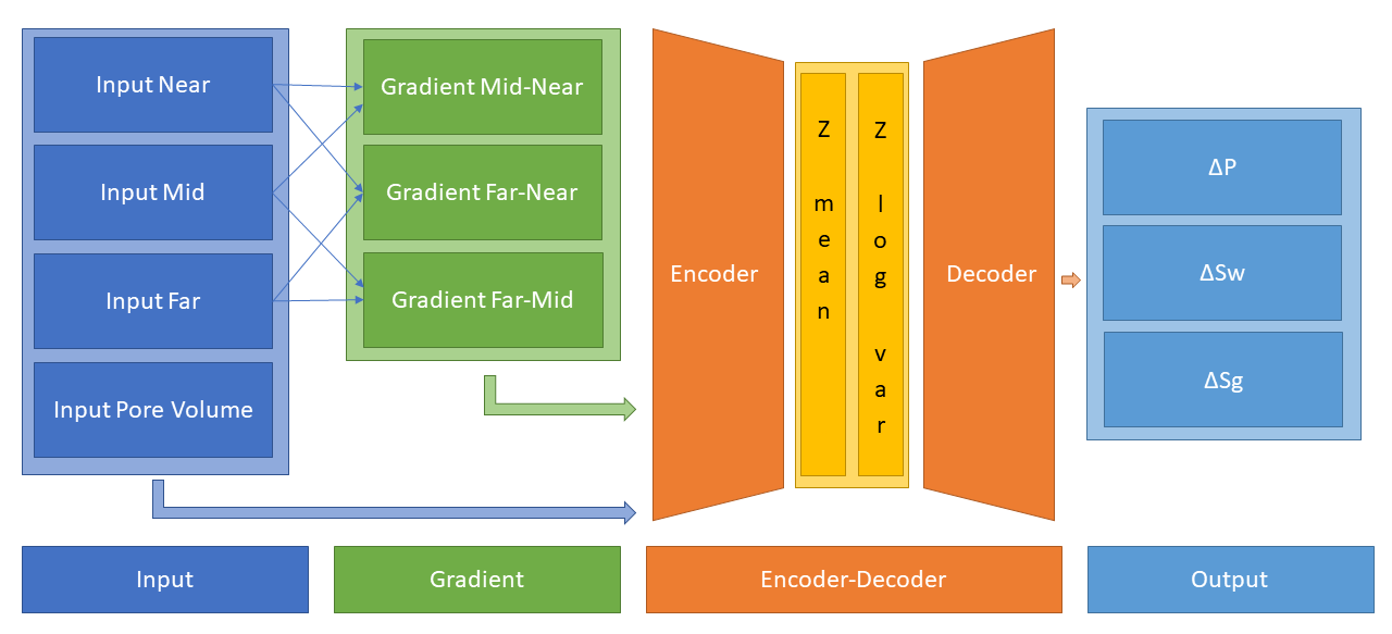
In Jesper Sören Dramsch, Corte, et al. (2019d) we present a novel network structure that explicitly includes avo gradient calculation within the network as physical knowledge, shown in 6.6.
The network architecture was chosen to follow an encoder-decoder architecture as a forcing function for information distillation. The encoder decreases in size with each layer, gradually compressing the input data, while the decoder decompresses the data to the designated output (Dony and Haykin 1995). Conventionally, the middle layer is called "bottleneck" or "code layer" as it contains the compressed representation of the input data. Encoder-decoder architectures have found wide application in neural network applications that necessitate data transformation to a different representation (Worrall et al. 2017).
Additionally, the bottleneck layer is implemented as a variational encoding layer to be less susceptible to noisy input. The specific implementation is based on variational auto-encoders (Diederik P. Kingma and Welling 2013). These replace the singular bottleneck layer with a number of layers that represent the parameters in a parametric probability distribution, most commonly the mean and variance of a Gaussian distribution \(\mathcal{N}\left(\mu, \sigma\right)\). The encoder then informs the Gaussian distribution at the bottleneck and the decoder samples from the distribution during training. At inference, these networks commonly return the mean of the distribution. Neural networks are conventionally trained using stochastic gradient descent, which is not well-behaved calculating the derivative of a random node. Diederik P. Kingma and Welling (2013) popularized the "reparameterization trick", which reformulates
with \(z\) being the bottleneck, \(P\) being the probability of the distribution \(\phi\) to approximate, and \(x\) being the data sample to
where \(g()\) is the functional representation of \(\phi\) parameterized by \(\mu\) and \(\sigma\) for a Gaussian distribution, and \(\epsilon\) being a random sample from \(\mathcal{N} (0,1)\) that is the source of randomness in the bottleneck layer computing as \(z = \mu + \sigma \cdot \epsilon\).
The pore volume is passed as-is to the network. The estimated pore volume helps the network to decouple the rock matrix from the fluid effects, which is further explored in 6.4. A schematic of the network is shown in 6.6, which shows the connections of the individual operations.
The network explicitly includes avo gradient calculation in the network architecture, considering it is physical knowledge we know will stabilize pressure and saturation change separation. Including basic physics knowledge leads to the network learning residual information, essentially defining another forcing function for the networks learning process. The avo gradient can be calculated explicitly as input to the network. However, performing the avo gradient calculation within the network enables programmatic augmentation of the input data during training. This implies that instead of learning one pre-computed avo relation, we can perform data augmentation of the input data and train on a significantly higher amount of correctly calculated avo gradients. This strategy can significantly improve the training strategy.
Training the Deep Neural Network for 4D Seismic Inversion
The model training is carried out in multiple phases. The first phase solely trains on un-augmented simulation data to determine an ideal network structure. The second phase trains on the fixed architecture with data augmentation to transfer the network to noisy field data. The network is optimized on standard mse while monitoring the R2-score.
The initial phase was carried out on simulation data with the data split into one part for training and a separate data set for validation. The seismic data from 2004 was held out as a test set. nas was applied to the network to determine depth and width of the architecture, using a tpe hyper-parameter search (J. Bergstra et al. 2015). This ensures an architecture in a controlled test environment on simulation data that is optimized for the complexity of the data.
In the second phase, to transfer the network to field data, the input of the network was combined with additive Gaussian noise (Chris M. Bishop 1995) to train the network for noisy field data input. The noise level was estimated in a manual process. Therefore, including the avo calculation within the network forces the network to learn noisy avo gradients that correspond to the augmented input. This process reduces the R2-Score and mse, which is an expected effect of noisy regression data (Hastie, Tibshirani, and Friedman 2009). Nevertheless, this produces consistent results on field data upon visual inspection.
The paper in 6.4 provides an ablation study, where parts of the neural network architecture are systematically switched off. Ablation studies are commonly used to explore and evaluate the effect of the individual components on the regression result. The paper in 6.5 shows the results of the deep neural network compared to a Bayesian inversion.
Workshop Paper: Including Physics in Deep Learning – An example from 4D seismic pressure saturation inversion
Introduction
Physics in machine learning often relies on transformations of data to beneficial domains and simulating additional data. Karpatne et al. (2017) show a physics-guided approach to model lake temperatures with neural networks. Schütt et al. (2017a) use deep neural networks to model molecule energies and Oliveira, Paganini, and Nachman (2017) employ a special architecture to capture scatter patterns in high-energy physics. When building deep learning pipelines, we can make informed choices in data modeling, but also build neural networks to maximize information gain on the available data. Ulyanov, Vedaldi, and Lempitsky (2018) has shown that the network architecture itself can be used as prior in machine learning. These approaches translate well to geoscience, where strong priors are often necessary to inform decisions.
Deep learning has revolutionized machine learning by replacing the feature generation and augmentation step by learned internal representations of features that maximize information gain. On image data analysis of these neural network filters have shown close relations to edge filters and color separators (Grün et al. 2016). Jesper Sören Dramsch and Lüthje (2018b) have shown that these filters translate well to seismic data. However, classic feed-forward neural networks do not have the benefit of learning filters. However, these neural networks benefit from recent improvements for regularization (Ioffe and Szegedy 2015), non-saturating and non-vanishing gradients (K. He et al. 2015), and training on GPUs.
Neural networks for inversion of seismic data have a long history (Roeth and Tarantola 1994). In (Jesper S. Dramsch et al. 2019) we show the application of a deep multi-layer perceptron for map-based 4D seismic pressure saturation inversion. In this work we show the information gain of feed-forward multi-layer perceptron neural networks by including an explicit calculation of the AVO gradient within the network architecture. It’s exemplary for including domain knowledge as a prior in machine learning.
Method
We build a deep feed-forward network to invert seismic amplitude maps
for pressure and saturation changes. We use the high-level Python
framework keras with a tensorflow backend. The neural network
was trained on synthetic data, to subsequently predict field data. The
network takes the seismic input samplewise with near, mid, and far
stacks, and pore volume. We inject 20% Gaussian noise to model the
noisier field data directly after the input layer. This is fed to a
custom layer that calculates the PP AVO gradient between far-mid,
mid-near, and far-near. The main components are as follows:
Gaussian noise injection
The synthetic model is noise-free. While we get good results on the training data and the modelled test data, the network does not transfer well to noisy field data. Although the 4D NRMS is very low in the data set, the sample-wise fluctuations in the field seismic differ significantly from the synthetic data. We apply additive Gaussian noise with \(\sigma = .02\) to the seismic inputs separately to simulate independent fluctuations of the seismic maps. This significantly decreases the training and validation performance on noise free synthetic data. On field data, however, this enables good transfer of the neural network.
Explicit AVO gradient calculation
The Schiehallion field is a good example of imbalanced learning. We have many samples of pressure changes \(\Delta P\), a good selection of water saturation changes \(\Delta S_w\), and very few gas saturation changes \(\Delta S_g\). Yet, the changes in gas saturation \(\Delta S_g\) produce the strongest changes in seismic P wave amplitudes. Statistically, these can easily be regarded as outliers, and therefore, possibly disregarded by the neural network. From decades of seismic analysis, we know that the AVO gradient is very good for pressure saturation separation. We implement an explicit calculation of AVO gradients in the network.
where \(G\) is the PP AVO gradient, \(A\) is the seismic P wave amplitude, \(x\) is the offset, and \(\Theta\) is the angle.
Encoder-decoder architecture
Subsequently, the four input maps and the three gradient maps are concatenated and fed to an encoder architecture that condenses the information to an embedding layer \(z\). This layer learns a collection of Gaussian distributions to represent the noisy input data The decoder samples this variational embedding layer to calculate the pressure change \(\Delta P\), change in water saturation \(\Delta S_w\), and gas saturation \(\Delta S_g\).
The full architecture is of the encoder-decoder class. The encoder reduces the number of parameters with each subsequent layer. This forces the network to learn a lossy compression of the input data as \(z\)-vector. The decoder increases the number of nodes per layer toward the output. The network therefore learns to correlate the low resolution representation with the desired output.
Full Architecture from Jesper S. Dramsch et al. (2019).
Variational Z Vector
The inversion of noisy input benefits from a variational representation of compressed z-vector. The networks learns Gaussian distributions in the embedding layer. Therefore, we have to apply the reparametrization trick outlined in Diederik P. Kingma and Welling (2013) to circumvent the sampling process cannot be learned by gradient descent. We use the implementation in Chollet and others (2015b) for variational autoencoders.
Results
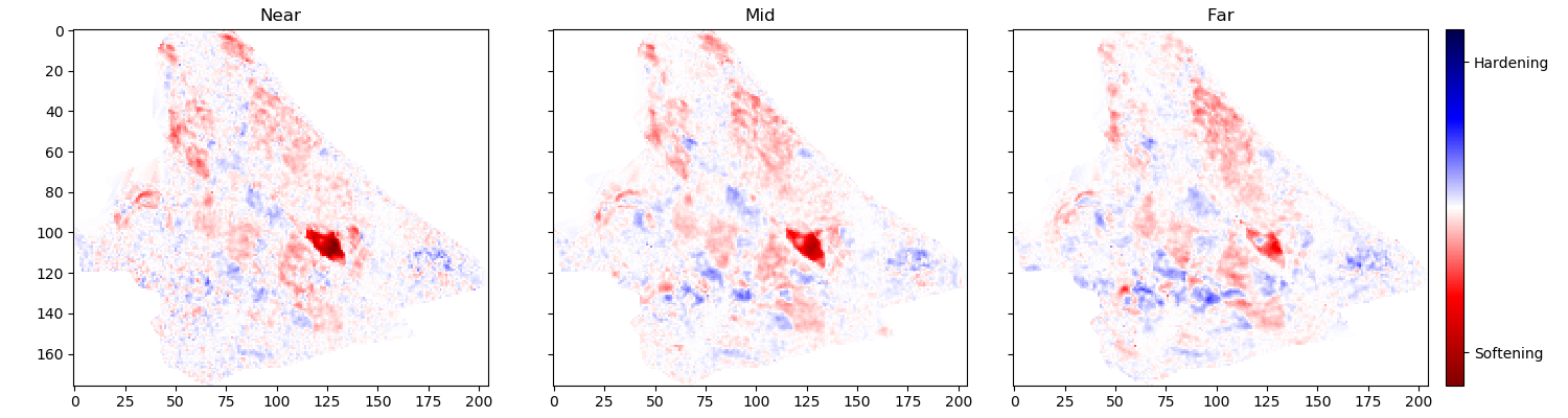
Schiehallion 2004 Timestep Seismic data, pore volume and sim2seis results.
In figure 6.2 we show the 2004 time step of the Schiehallion 4D. Figure 6.3 contains the inversion result using the variational encoder decoder architecture. Some coherency in the maps can be seen, but each map is very noisy and the gas saturation map contains many data points that indicate gas desaturation, which cannot be confirmed by production data.
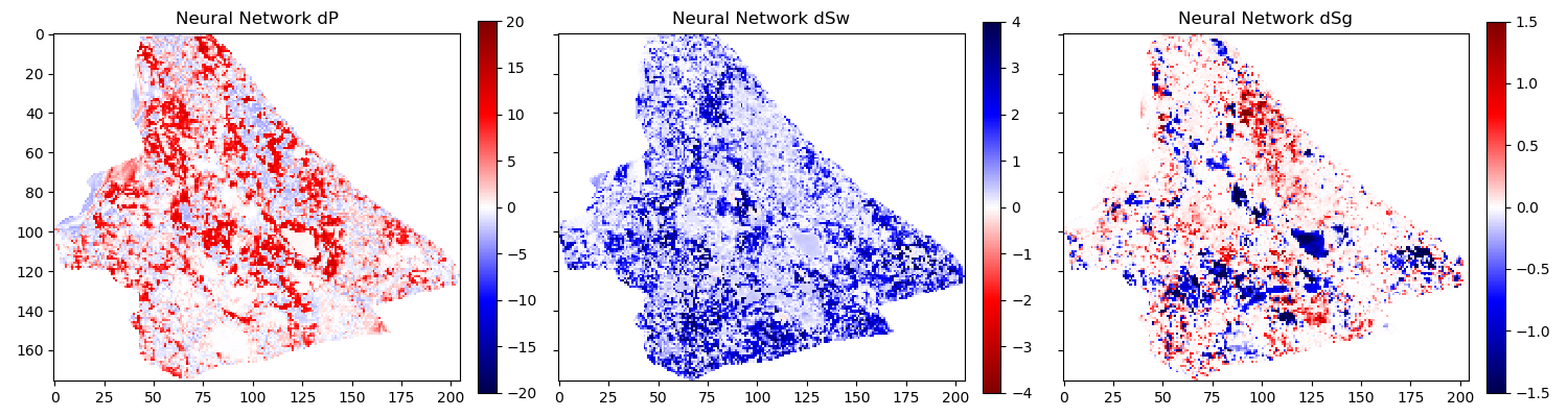
Variational Encoder Decoder Architecture Inversion
When we add the gradient, we can clean up some of the misfit in the gas saturation maps \(\Delta S_g\). Particularly, the event with the strongest softening in the amplitude maps, is partially reassigned to the pressure map \(\Delta P\). However, the inversion process is still very prone to noise. In figure 6.5, we show the inversion results of a AVO-gradient neural network with a noise injection at training of \(\sigma = .02\). The inversion maps are very coherent. Noise injection without gradient calculation does not give adequate results.
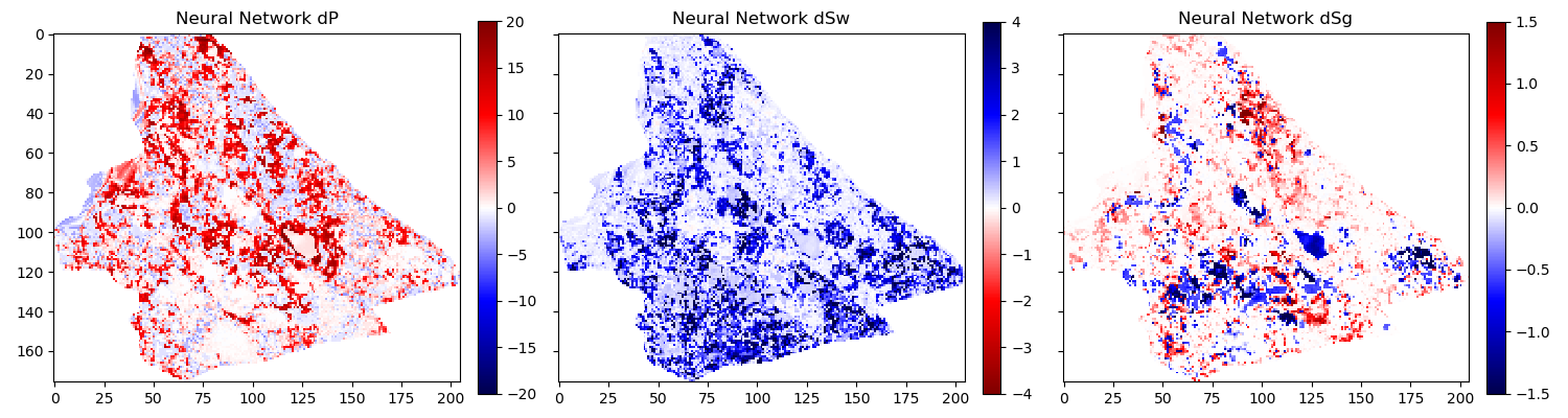
AVO-Gradient Variational Encoder Decoder Architecture Inversion
Noiseinjected AVO-Gradient Variational Encoder Decoder Architecture Inversion
Conclusions
We have shown a neural network architecture that incorporates physical domain knowledge to enable transfer from synthetic to field data. The final inversion result has very good coherency, despite the network not having any spatial context. While further investigation is necessary, this indicates that useful information has been learned. This is one example, where bias can be intentionally introduced into the network architecture to include physics into machine learning.
Acknowledgements
The research leading to these results has received funding from the Danish Hydrocarbon Research and Technology Centre under the Advanced Water Flooding program. We thank the sponsors of the Edinburgh Time-Lapse Project, Phase VII (AkerBP, BP, CGG, Chevron, ConocoPhillips, ENI, Equinor, ExxonMobil, Halliburton, Nexen, Norsar, OMV, Petrobras, Shell, Taqa, and Woodside) for supporting this research. The Brazilian governmental research-funding agency CNPq. We are also grateful to Linda Hodgson and Ross Walder for important discussions on the field and dataset.
Workshop Paper: Deep Learning Application for 4D Pressure Saturation Inversion Compared to Bayesian Inversion on North Sea Data
Introduction
Estimating reservoir property change during a period of production from 4D seismic data has been a concentrated challenge and ambition for geoscientists in the oil and gas industry. These estimates can contribute to a better history matching of the reservoir simulation and for more comprehensive reservoir monitoring.
With the advance of machine learning techniques on all fronts in the geosciences we can address what roles machine learning can take in the established pressure and saturation inversion workflows and what other new workflows can be constructed using this tool. Machine learning is such a broad concept that it can be incorporated at different levels on all the current well established workflows to diminish their weaknesses, bringing more value to the pressure and saturation estimations from seismic inversion. Not only that, with this tool we can create completely new workflows that we are only beginning to grasp.
Here we will present results for two separate methodologies of seismic inversion to changes in pressure and saturation. The first method is a well established model-based Bayesian inversion method using a calibrated petro-elastic model and convolution workflow as the forward seismic modeling operator. In the second method we use a deep neural network to model the inversion process, we use synthetic seismic data to train the network, then apply the inversion to observed data. The methods are applied to the same field data giving a nice platform to compare the neural network inversion results to a more conventional approach.
Schiehallion Data
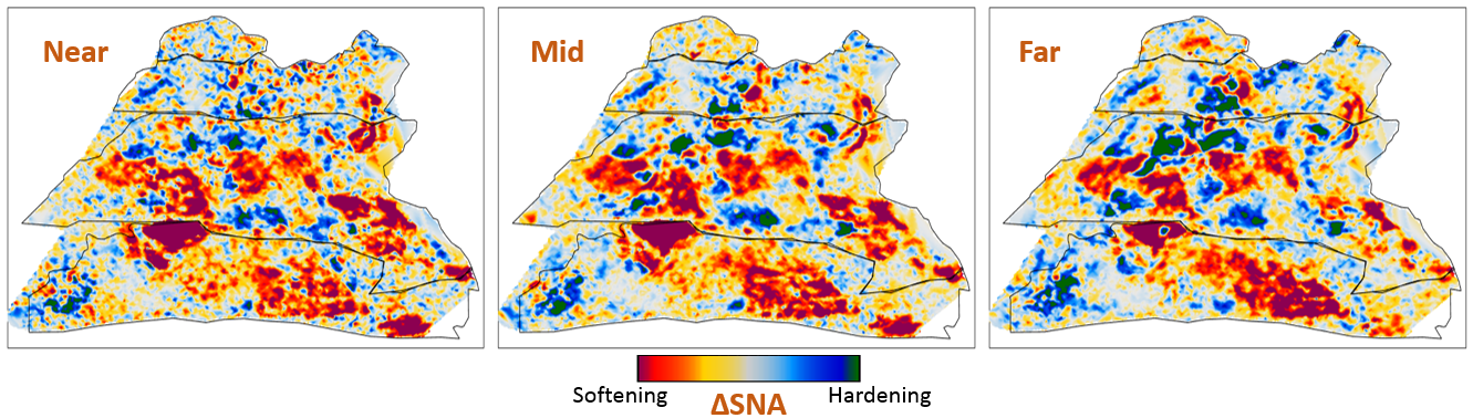
The inversions are applied to maps of Schiehallion’s upper T31 sandstone. It is a fairly thin reservoir (5-30m), which is well defined in the seismic data by one single trough. For this reason, a map-based approach is appropriate. Schiehallion is a highly compartmentalized field with initial pressure close to bubble point pressure. Production in this complex structure led to areas with strong pressurization due to water injection into closed compartments, while other areas lack the pressure support and experience gas release due to pressure depletion. We face the challenge of inverting 4D seismic data to changes in pressure, water saturation and gas saturation (\(\Delta\)P, \(\Delta\)Sw and \(\Delta\)Sg), so the methods need to deal properly with the non-linearities due to each of these effects. The seismic data analysed is a set of eight vintages (from 1996 to 2010). These were reprocessed by CGG in 2014, following a 4D driven multi-vintage workflow. The processing workflow was carefully optimized to maintain 4D AVO amplitudes intact. Synthetic feasibility studies showed that the 4D AVO attributes are in line with the theoretical expectations. The seismic data used for inversion is the 4D difference of the sum of negative amplitudes (\(\Delta\)SNA) map attribute, extracted from three angle-stacks, along the reservoir time window (see figure 6.7).
Method 1 - Model-based Bayesian inversion
The Bayesian invesion workflow is explained in detail in Gustavo Corte, MacBeth, and Amini (submitted 2019). Essentially the workflow uses a petro-elastic model calibrated to the seismic data by H. Amini (2018) and a convolutional step to model the seismic data. The \(\Delta\)SNA attribute is then extracted from the synthetic seismic and compared to the real seismic \(\Delta\)SNA map. Since this is a map-based inversion, all realizations are sampled in map form and then go through a conversion into the vertical reservoir simulation grid in order to run the forward modelling process. We use a monte carlo sampling algorithm to generate thousands of realizations of the full map and from these extract best estimations and uncertainties. This inversion is constructed in a Bayesian model-based form, with the objective of bringing together information from the history matched reservoir simulation and seismic data. Reservoir simulation results for \(\Delta\)P, \(\Delta\)Sw and \(\Delta\)Sg are incorporated as prior knowledge, to settle ambiguities and lack of seismic information. Where the seismic data lacks information about a certain property the method will bring this information from the simulation model. The inversion results will deviate from the simulation in areas where the seismic data contains enough consistent information to indicate an update is necessary.
Method 2 - Neural network inversion
We use a deep neural network to model the inversion process, based on the synthetic convolution seismic data. Although convolutional neural networks are considered the state of the art in spatially correlated data, we show that a sample-wise feed forward neural network trained on noise-free convolutional seismic can invert observed seismic data. We aim to build a regression model that can invert physical seismic angle stack data to pressure and saturation data.
Distinguishing pressure and saturation changes in 4D seismic data is a
hard to solve problem. In neural networks, this is no different. The
variation of data showing different pressure and saturation change
scenarios is sparse, which complicates training and may possibly be
disregarded as noise. This increases the need for training data
immensely. However, we can include prior physical insights into neural
networks to reduce the cost of training and uncertainty. As neural
networks are at its basis very large mathematical functions, we can
explicitly calculate the P-wave AVO gradient within the network to use
as additional information source, without the need of feeding it into
the network as input data. This has the added benefit of the network
learning on noisy gradients. The design choice for the neural networks
can be arbitrary, however, encoder-decoder networks have proven to force
neural networks to find meaningful relationships within the data and
reduce to these in the bottleneck or embedding layer. For the final
architecture we used hyperopt (J. Bergstra, Yamins, and Cox 2013)
and keras (Chollet and others 2015b). This allows us to use a Tree
of Parzen (TPE) estimator for hyperparameter estimation. The estimator
models \(P(x|y)\) and \(P(y)\), where \(y\) the quality of
fit and \(x\) is the hyperparameter set drawn from a non-parametric
density (J. S. Bergstra et al. 2011).
Architecture for sample-based seismic inversion with explicit gradient calculation.
The architecture is shown in figure 6.6. Inputs are Near, Mid, Far seismic, and Pore volume. These Input Layers are passed on to calculate the mid-near, far-mid, and far-near gradients. These four inputs and three gradients are concatenated and fed to the encoder. z_mean and z_log_var build the variational embedding with z_Lambda being the sampler fed to the decoder network. The decoder splits into three output layers \(\Delta\)P, \(\Delta\)Sw, and \(\Delta\)Sg.
The network is trained using sim2seis results calculated for the seven time-steps at seismic monitor acquisition times, it is then used to invert each seismic monitor individually. The inversion results for the synthetic data gave a consistent \(R^2\)-score of over 0.6 for all simultaneous inversion targets \(\Delta\)P, \(\Delta\)Sw and \(\Delta\)Sg with an encoder-decoder architecture and a deterministic embedding layer. While we kept the main architecture constant, we replaced the embedding layer with a variational formulation to allow for noise in the input to output mapping added noise injection to the input layer, to apply Gaussian Noise during the training phase. This significantly improved the inference on observed seismic data. The total training time for the network was 3 hours on a K5200 GPU, prediction speed takes \(5.11~s \pm 22.1~ms\).
Schiehallion Field Data Example
The field data differs significantly from the synthetic data in that it is noisier, assuming the same ground truth. This is a true challenge for a sample-wise process to produce consistent results. We have trained the network with Gaussian noise on the input data with zero mean and a standard deviation of \(\sigma = .02\), therefore, approximately \(95~\%\) of the noise may distort up to a maximum \(40~\%\) of the clean signal.
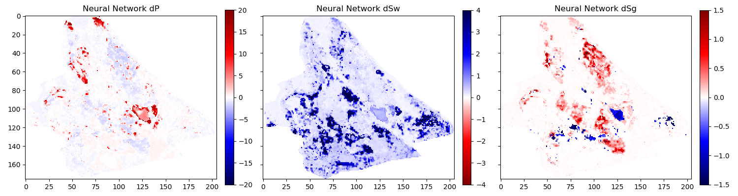
Figure 6.7 shows the observed 4D seismic maps (\(\Delta\)SNA) for the 2004 monitor acquisition using the 1996 acquisition as baseline. Figure 6.8 shows, in the first row, the simulation model results (used in the Bayesian method as prior information), in the second row, the inversion results for the Bayesian method, and in the third row, the inversion results for the neural network method.
Schiehallion 2004 Timestep Seismic data, pore volume and sim2seis results.
From figure 6.8 we can see clearly the influence of the prior simulation model in the Bayesian results. The neural network does not use a prior, so the results are not influenced by the simulation model and can be seen as a direct interpretation of the seismic data. Comparing both we can see what bits of information the Bayesian method is bringing from the prior. The seismic data is most sensitive to gas saturation changes, so the Bayesian method is able to capture this consistent information from seismic data and deviate \(\Delta\)Sg results from the initial prior. The results for gas saturation are the most in agreement in both methods precisely because all this information is coming from the seismic data. We see some leakage of hardening effects into the \(\Delta\)Sg results in method 2 due to the fact that we cannot set constraints to that inversion process. Since there is no initial gas saturation in those areas the saturation change cannot be negative, these comprehensive constraints are imbedded into the Bayesian workflow but not in the neural network.
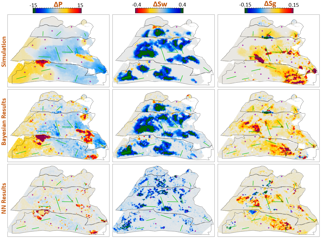
Schiehallion 2004 Timestep Bayesian Inversion and Neural Inversion
Water saturation has a distinctive hardening effect on seismic data, but in this map it is highly obscured by stronger overlying softening effects due to pressure increase and gas breakout. The neural network interprets all the hardening anomalies correctly as water saturation increase, while controlling for noise in areas of softening amplitudes. In those areas the seismic data does not contain useful information on the water saturation so the Bayesian result relies on a strong prior to compensate. All of the water saturation inverted by method 2 is in agreement with method 1, but since method 1 has this additional information from the prior, the map seems more coherent.
The pressure effect on seismic is highly non-linear. While high increases in pressure show a very strong softening effect, milder pressure variations (up to \(\pm7~MPa\)) have very little influence on the seismic data and are easily obscured by overlying effects. For this reason, the neural network pressure inversion in regions of mild change is low and often correlated with saturation. The Bayesian inversion benefits from the prior to fill those pressure values. This method does deviate from the prior in areas of strong softening signals due to pressure increase, and those areas are also correctly interpreted by the neural network inversion.
When we relax the prior of the Bayesian inversion, these results are very noisy in the pressure and water saturation estimates. In these areas the neural network inversion is robust to noise. During the neural network training the pore volume has shown to be important in guiding the inversion from the seismic data. Adding pore volume data adds a structural component to the neural inversion process, which improves the overall results from the sample-based method significantly.
Conclusions
This work presents Deep Neural Inversion of 4D seismic data. We compare the results with a Bayesian Inversion approach. We show that Deep Neural Networks can model seismic inversion trained on synthetic data. Explicit calculation of the P-wave AVO gradient within the network stabilizes the pressure-saturation separation within the network and Noise Injection enables the transfer to unseen seismic field data. Neural networks can be an important tool to investigate nascent information in 4D seismic data to improve inversion workflows and reduce uncertainty in seismic analysis.
The Neural Inversion can be used as a valuable tool to explore purely data-based inversion results in the presence of noise. It is able to translate the ambiguous seismic amplitudes into much more easily interpreted property maps. The value of the Bayesian inversion results presented is in combining all knowledge about the reservoir to create a general view of the reservoir dynamics. These results show the current understanding of reservoir dynamics updated by imprinting seismic information on top of the history matched simulation results.
Acknowledgements
The research leading to these results has received funding from the Danish Hydrocarbon Research and Technology Centre under the Advanced Water Flooding program. We thank the sponsors of the Edinburgh Time-Lapse Project, Phase VII (AkerBP, BP, CGG, Chevron, ConocoPhillips, ENI, Equinor, ExxonMobil, Halliburton, Nexen, Norsar, OMV, Petrobras, Shell, Taqa, and Woodside) for supporting this research. The Brazilian governmental research-funding agency CNPq. We are also grateful to Linda Hodgson and Ross Walder for important discussions on the field and dataset. We thank Mikael Lüthje for valuable feedback.
Discussion of 4D Inversion
The workshop paper Jesper Sören Dramsch, Corte, et al. (2019a) contains the neural network results compared to the simulation and Bayesian inversion results, shown in 6.8. This network does not calculate the inversion solution; it merely approximates the inverse problem. These initial results on limited training data show that a neural network can estimate pressure saturation information from field data, after training on simulation data.
The results presented in 6.8 contain three indicators that the network learned a regression for the Schiehallion field. The network returns the overall trend in increase and decrease of pressure and saturation correctly. Additionally, the range of output values for the network is unconstrained, but the network calculates values in the ranges that are expected from the simulation and Bayesian inversion results. However, and more interestingly, the networks do not contain spatial information, being a feed-forward dnn not a convolutional neural network, yet returns continuous albeit noisy outputs when re-assembled into maps.
While the overall result is promising, regions of strong gas saturation changes present a problem. This could be due to problems in the modelling, as well as the fact, that they generate strong amplitude differences and are far in between, essentially behaving like outliers.
Contribution of this study
This study introduced a dnn to approximate a 4D qi pressure-saturation inversion problem with a regression model. The contribution of this study is threefold in that it approximated the pressure-saturation inversion, included physical information in the network, and trained on simulation data and transferred to field data. The work included in this thesis are two workshop papers (Jesper Sören Dramsch, Corte, et al. 2019d, 2019a); however, a journal paper (Côrte et al. 2020) and conference paper (G. Corte et al. 2020) have been published, resulting directly from this work.