3D Time Warping for 4D Data
Dramsch, J. S., Christensen, A. N., MacBeth, C., & Lüthje, M. (2019, October 31). Deep Unsupervised 4D Seismic 3D Time-Shift Estimation with Convolutional Neural Networks. https://doi.org/10.31223/osf.io/82bnj |
||

This chapter consists of the submitted journal paper (Jesper Sören Dramsch, Christensen, et al. 2019). This paper presents a novel 3D warping technique for the estimation of 4D seismic time-shifts. The algorithm is unsupervised and provides 3D time shifts with uncertainty measures. The unsupervised nature of this algorithm avoids biasing the ml model with ground truth data from existing time-shift extraction algorithms.
4D seismic time shift extraction is often performed in 1D due to time constraints and often sub-par performance of 3D algorithms (P. Hatchell and Bourne 2005). In geologically complex systems and pre-stack time-shifts, these simple approaches often break down and obtaining 3D time-shifts is beneficial. This chapter explores and summarizes conventional 3D warping methods and machine learning approaches. The paper Jesper Sören Dramsch, Christensen, et al. (2019) in this chapter adapts the medical Voxelmorph algorithm to match 4D seismic data volumes in 3D.
Common 1D approaches include local 1D cross-correlation, dynamic time warping (Dave Hale 2013a), optical flow methods and methods based on Taylor expansion (Zabihi Naeini et al. 2009). 3D methods include Dynamic Image Warping (DIW) (D. Hale 2013), which expands dynamic time warping to two and three dimensions respectively. DIW is, however, at its core a depth-wise method that then gets smoothed across trace-wise matches. 3D local cross-correlation defines a multi-dimensional cross-correlation in a fixed Gaussian window to make the problem computationally feasible. The method requires processing of the seismic images to perform reasonably, usually smoothing and spectral whitening. J. Rickett, Duranti, Hudson, et al. (2007) introduce a non-linear inversion-based time-shift extraction in 3D. Cherrett, Escobar, and Hansen (2011) further develop a geostatistical inversion combining data constraints with geostatistical information in a Bayesian inversion scheme.
Zitova and Flusser (2003) review the rich history of medical registration methods that partially overlap with 4D seismic methods. These methods include affine transformations, piece-wise linear transformations (Goshtasby 1988), radial basis function-based methods (Zitova and Flusser 2003), and elastic deformations (Bajcsy and Kovačič 1989). The method most relevant to this paper is lddmm (Beg et al. 2005), which has not found application in 4D seismic, due to being computationally expensive. The method finds a combination of diffeomorphisms, which will be introduced in 16.1, through the deformation field of two images. lddmm then finds the shortest path of these diffeomorphisms iteratively.
Diffeomorphisms
In simple terms a diffeomorphism is a smooth transformation of an image, i.e. no discontinuities or holes are introduced. In the following we will constrain ourselves to \(\mathbb{R}^3\) for brevity’s sake. We define two images \(B, M\) and assume \(B\) is a random deformation of \(M\), then \(B \in \mathcal {B} := \{ B=M \circ \varphi, \varphi \in {Diff}_V \}\), with \(\varphi\) being a diffeomorphic flow from \({Diff}_V\). Diffeomorphisms in \(\mathbb{R}^3\) are a group of bijective, smooth transformations of local areas in dense images generated as smooth flows \(\phi_t, t \in [0,1]\), with \(\varphi := \phi_1, \phi_0 := \text{id}\) (Beg et al. 2005). They satisfy the Lagrangian and Eulerian specification of the flow field for diffeomorphisms associated with the ode
with \(\phi\) being the smooth flow, where \(\dot{\phi}_t \in \mathbb{R}^3\) are the Lagrangian vector fields and \(v\) the Euclidean velocities of the system. \(\phi_0\) is determined to be the identity transformation. Beg et al. (2005) approached this problem as a variational problem, whereas M. I. Miller, Trouvé, and Younes (2015) reformulated as a Hamiltonian optimal control problem on the variational objective. The variational objective for densely matched images \(B\) and \(M\) as is the case in seismic data following can then be defined as minimizing the Cost \(C\) of a given vector field \(v\)
for images B, M: \(\mathbb{R}^3 \rightarrow \mathbb{R}^+, \phi\cdot B \colon=B\circ\phi^{-1}\). Here \(A\) is the one-to-one matrix linear differential operator such that \(A: V \rightarrow V^*\), which enforces the smoothness constraint by modelling the norm \((V, \Vert\cdot\Vert_V)\). \(\sigma\) represents vector elements in the dual space \(V^*\), which in this case are generalized functions which represent the conjugate momentum representations of the system. They act on smooth vector functions \(f \in V\) further following M. I. Miller, Trouvé, and Younes (2015) to provide energy with \((\sigma | f) \colon= \int_X\vec{f}(x)\cdot\vec{\sigma}(dx)\). It follows that \(A v\) can be interpreted as the Eulerian momentum. Allowing \(A v\) to be singular implies that coordinates can be displaced homogeneously by a singular momentum. Then [eq:diffeomorphism] can be interpreted as minimizing two objectives, namely the action integral of kinetic energy and the endpoint matching. This is equivalent to finding the aforementioned shortest path of diffeomorphisms, while matching the resulting image as closely as possible.
Image Matching Algorithms
Machine learning-based methods within computer vision are mostly applied in image- and video-processing applications. Supervised methods largely work off the assumptions in Optical Flow (Dosovitskiy et al. 2015; Ranjan and Black 2017). FlowNet (Dosovitskiy et al. 2015) implements an Encoder-Decoder convolutional neural network architecture. It has reached wide reception in the field, and several modifications were implemented; namely, FlowNet 2.0 (Ilg et al. 2017) improving accuracy, and LiteFlowNet (Hui, Tang, and Change Loy 2018) reducing the computational cost. SpyNet (Ranjan and Black 2017) and PWC-Net (D. Sun et al. 2018) implement stacked coarse-to-fine networks for residual flow correction. PatchBatch (Gadot and Wolf 2016) and deep discrete flow (Güney and Geiger 2016) implement Siamese Networks (Sumit Chopra et al. 2005) to estimate the optical flow. Alternatively, DeepFlow (Weinzaepfel et al. 2013) attempts to extract large displacements optical flow using pyramids of sift features. These methods are prone to the same problems classic optical flow algorithms exhibit. Moreover, supervised methods necessitate ground truth time shifts. This leads to two problems; Either the model needs to be trained on synthetic data, where shifts are known and transfer model to field data, or we need to train the network on time shifts extracted by a different method. The implication of training a deep neural network on data extracted by a different method trains the network to include all assumptions the extraction methods make. Training on time shifts extracted by a 1D method would, therefore bias the network to return pseudo-trace-wise predictions.
Unsupervised methods include different approaches to the problem of image- and volume-matching. Meister, Hur, and Roth (2018) modifies the FlowNet architecture to an unsupervised optical flow estimator with bidirectional census loss called UnFlow. UnFlow makes several changes to the original optical flow formulation, which relax the illumination constraint (Stein 2004). Bansal et al. (2018) implements a cycle-consistent generative adversarial network (Cycle-GAN) to interpolate video frames. This method is potentially promising but falls short due to training data constraints in seismic data. Video data contains at least 24 frames per second of video, which provides training data. One second of video, therefore, already contains more time steps than the best-covered field in 4D seismic data. Voxelmorph (Balakrishnan et al. 2019) implements a U-net (Ronneberger, Fischer, and Brox 2015b) within an architecture that extracts a static velocity field, which is integrated to obtain a diffeomorphic warp field and performs a 3D interpolation to match the fields and trains unsupervised. This method significantly reduces the underlying assumptions necessary to make the network perform well on seismic data. The Voxelmorph algorithm is based on the diffeomorphic assumption, which constrains the solution space of the mapping. The main benefit of applying the diffeomorphic mapping to geoscience data comes in the fact that all diffeomorphisms are homeomorphic. The homeomorphic assumption transfers well to the geological reality that the mathematical topology stays constant, resulting in reflectors neither crossing nor generating loops.
The paper in (Jesper Sören Dramsch, Christensen, et al. 2019) applies the Voxelmorph architecture in Dalca, Balakrishnan, Guttag, et al. (2018) to 4D seismic data. I make the network work on seismic data and train it on the Dan 1988-2005 seismic volumes in 3D. Seismic data is significantly larger than most brain scan data, which necessitates patch-based training of the network. I compare the obtained warp field to the best match, I could obtain using classic methods on the available data. The DIW match is sufficiently similar to the Voxelmorph warping field to warrant further investigation. The Voxelmorph architecture implements a subsampled flow field, which I replaced by a full U-Net that provides full-scale 3D flow fields with uncertainties. The paper includes an investigation of the differences between the subsampled and full-scale flow fields. Moreover, I validate the unsupervised model on the same field with different seismic data, collected at different times, with differing seismic acquisition equipment, including different azimuths. Moreover, I test the model on a seismic data set from a different field, with different geology, acquisition, and year. Finally, the machine learning approach is compared to a time-shift field obtained with diw.
Dynamic Time and Image Warping
The paper in Jesper Sören Dramsch, Christensen, et al. (2019) uses dtw but does not expand on the method; hence an introduction to the algorithm is presented here. dtw is a signal processing tool for time series with the capability to match arbitrary time-series. Within geophysics it is applicable to 4D time shifts, seismic-well ties, well-to-well ties, and seismic pre- and post-stack migration (Hale2013; Luo2014). dtw itself is a dynamic programming problem described in [Algorithm 1].
 |
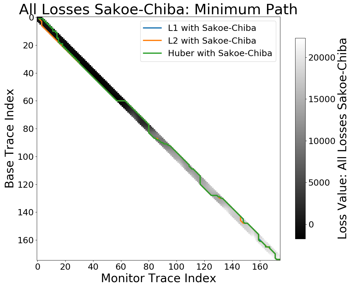 |
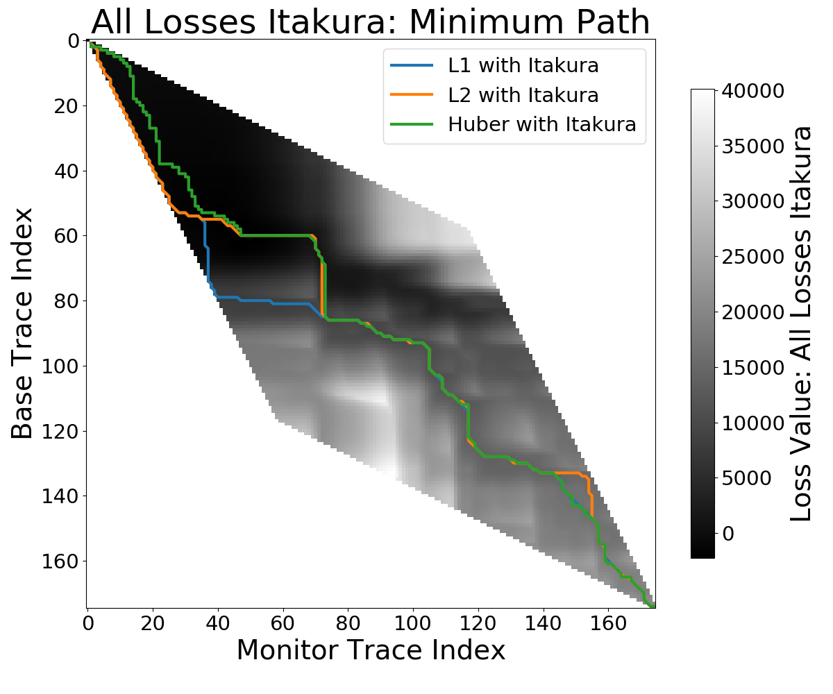
Figure 7.1: Minimum path for constraint masks for cumulative cost in DTW. Images show the optimum path for different loss functions, including L1, L2, and the Huber loss.
The dtw algorithm, represented in [dtw], relies on calculating a distance matrix sample-wise between two traces \(a\) and \(b\). Commonly, the \(L_1\) norm is used to calculate the distance with \(|b-a|\). Alternatively, the euclidean distance or \(L_2\) norm can be used, which modifies the calculation to \((b-a)^2\). The difference between \(L_1\) and \(L_2\) is significant in the sense that the \(L_1\) norm is not differentiable or convex; however, it scales linearly for outliers. The \(L_2\) norm converges fast close to zero; however, the error "explodes" for outliers. The Huber loss from convex optimization combines the advantages of the \(L_1\) norm and \(L_2\) norm
which is convex for small values, scales linearly for outliers and is differentiable for all values of \(\mathbb{R}\), with \(\delta\) being a scaling factor.
Algorithm: DTW(a, b)
Given: Trace `a` and Trace `b` of lengths `n`.

Function CalculateDistanceMatrix(a, b)
   D ← dist(a, b)
   return D

Function CalculateCumulativeCost(D)
   C[0,0] ← 0
   for i = 1 to n  # Populate Edge
      C[0,i] ← D[0,i] + C[0,i-1]
      C[i,0] ← D[i,0] + C[i-1,0]

   for i = 1 to n  # Fill Cumulative Cost Matrix
      for j = 1 to n
         C_min ← min(C[i,j-1], C[i-1,j-1], C[i-1,j])
         C[i,j] ← D[i,j] + C_min
   return C

Function BacktrackMinimumCostPath(C)
   P ← C[n,n]
   while i > 0 or j > 0
      i, j ← index(P[last])
      C_min ← min(C[i,j-1], C[i-1,j-1], C[i-1,j])
      P.append(index(C_min))
   return P

D ← CalculateDistanceMatrix(a, b)
C ← CalculateCumulativeCost(D)
P ← BacktrackMinimumCostPath(C)

return P
Algorithm 1: Dynamic time warping algorithm consists of calculating the element-wise distance matrix, cumulative cost and then find the optimal path in the cumulative cost matrix
Additionally, the search space on the cumulative distance matrix can be constrained to both increase performance and avoid non-optimal solutions. The different global constraint strategies are presented in [fig-constraints]. The Itakura parallelogram (Itakura1975?) in [fig-itakura] describes a parallelogram that has the largest width across the diagonal of the matrix, providing the highest degree of flexibility for the dtw algorithm in the centre parts of the seismic traces. The Sakoe-Chiba disc (Sakoe1978?) follows a different strategy, which provides a constant maximum warp path. This strategy in [fig-sakoe] introduces a global maximum time shift. Other constraints on the warp path in dtw are local rate changes that limit the local changes, also called step patterns (Sakoe1978?; Giorgino and others 2009).
diw is the extension of dtw to 2D and 3D datasets. (Hale2013?) introduced DIW for seismic data by applying the DTW algorithm in z-direction along the time-series and smoothing adjacent time-shifts to obtain consistent results. This process can be done iteratively with progressively smaller smoothing windows to obtain x-y consistent DIW results. It is important to note that DIW does not increase the computational cost of the DTW algorithm itself. Contrary to the intuition, the distance matrixes and cumulative cost presented in the are calculated in the same way resulting in a 2D cost matrix for each pair of 1D time series. However, the amount of comparisons of traces increases in 2D and 3D, scaling up the computational cost.
Journal Paper: Deep Unsupervised 4D Seismic 3D Time-Shift Estimation with Convolutional Neural Networks
Introduction
Seismic time-lapse data consists of two 3D reflection amplitude cubes that represent the subsurface they were collected from. These cubes are acquired years apart with expected changes in the subsurface due to e.g. hydrocarbon production. The differences in the subsurface cause changes in both amplitudes and velocities, which introduces misalignment of seismic reflectors. Measuring the misalignment and aligning these surfaces to obtain a reliable difference cube is one of the main disciplines in 4D seismic processing.
These time shifts are most commonly obtained by windowed cross-correlation and other statistical or signal processing approaches (MacBeth, Mangriotis, and Amini 2019). Considering the recent advances of machine learning in imaging and domain transfer, we explore possibilities of alignment with convolutional neural networks. Machine learning approaches, however, most commonly require labeled data to find a mapping \(f(x) = y\), with \(x\) being the input data, \(f\) being the blackbox algorithm like a neural network, and \(y\) being the labels or target.
A common problem in machine learning for subsurface science is determining the ground truth. Obtaining information from the subsurface is often prohibited by cost, and e.g. core samples are highly localised data that is often altered by the extraction method as well as the sheer act of unearthing the sample. Additionally, synthetic data may introduce the inverse crime (Wirgin 2004) of using the same theory to generate and invert data. Luckily, the physics of medical imaging and inversion is very similar to geophysics, where methods can be validated and fine-tuned. The main method discussed in this paper is adapted from the medical imaging literature.
The lack of ground truths leads to another problem that deep learning address but do not solve. For classic neural networks, we need to know a target label dataset, i.e. knowing a prior warp velocity. In 4D seismic this would mean employing an established method to obtain time shifts. This would effectively result in abstracting that method in a neural network, or modelling the warp, which would lead to committing the inverse crime. Logically, this lead us to explore unsupervised methods.
We discuss several options for architectures for mapping the monitor seismic cube to the base seismic cube directly within the network. This is possible in unsupervised configurations but depending on the architecture of the network this problem can be ill-constrained and generate non-physical mappings. One warranted criticism of deep learning and neural networks is the lack of explainability and limited interpretability. However, we employ a deep neural network to obtain warp velocity vectors, a 3D equivalent of time shifts, for dense deterministic warping instead of directly obtaining the warped result from a neural network. This enables us to interpret the warping vectors and constrain the warp path in addition to the warp result.
Moreover, we present the first 4D seismic 3D time shift estimator with uncertainty measures. We achieve this by implementing a variational layer that samples from a Gaussian with the reparametrization trick (Durk P. Kingma, Salimans, and Welling 2015). Therefore, we can counteract some of the influence of noise on the performance of the network.
Theory
Extracting time shifts from 4D seismic data is most commonly done trace-wise (1D), which limits the problem to depth. This provides sufficient results for simple problems. However, geologically complex systems and pre-stack time shifts benefit from obtaining 3D time-shifts. We discuss classical 3D time-shift extraction methods, we then go on to discuss relevant deep learning methods. These methods extract time-shifts with different constraints which we explore. For brevity we present the results of the best method to date, developed for the medical domain: VoxelMorph (Balakrishnan et al. 2019).
The goal of both conventional and machine learning methods is to obtain a warp velocity field \(\textbf{u}(x,y,z)\) that ideally aligns two 3D cubes \(B\) and \(M\) within given constraints. That means a sample \(m[x,y,z]\) will be aligned by adjusting \(m[x+u_x,y+u_y,z+u_z]\). In image processing this is considered "dense alignment" or "dense warping", hence we need a dense vector field to align each sample in the base and the monitor cube. Generally, \(\textbf{u}(x,y,z) \in \mathbb{R}^3\), which implies interpolation to obtain the warped result.
Conventional Methods
Most conventional methods in 4D seismic warping focus on 1D methods (P. Hatchell and Bourne 2005), which include local 1D cross-correlation, dynamic time warping (Dave Hale 2013a), optical flow methods and methods based on Taylor expansion (Zabihi Naeini et al. 2009). We do not cover these methods in detail, but focus on the limited applications of 3D methods in 4D seismic warping.
Local 3D Cross Correlation
Hall et al (S. A. Hall et al. 2005) introduced local 3D cross-correlation as a method for surface-based image alignment. The horizon-based nodal cross-correlation results were then linearly interpolated to full cubes. Hale et al (Dave Hale 2006) extended this method to full seismic cubes by calculating the multi-dimensional cross-correlation windowed by a Gaussian with a specified radius. The correlation results are normalized to avoid spurious correlations by amplitude fluctuations and high-amplitude events. Subsequently the cross-correlation result is searched for peaks using the following triple sum:
with \(c\) being the cross-correlation lag. The computational complexity of this method is \(\mathcal{O}(N_s \times N_l)\) with \(N_s\) being the total number of samples and \(N_l\) being the total number of lags.
Stabilization of the results of 3D cross-correlation is obtained by applying spectral whitening of the signals and smoothing the images with a Gaussian filter without increasing the computational complexity despite the windowing function (Dave Hale 2006).
Inversion-based methods
Rickett et al (J. Rickett, Duranti, Hudson, et al. 2007) describe a non-linear inversion approach, with the objective function being
with m being the model vector, d being the data vector. The non-linear inversion is constrained by applying the first-derivative to the spatial dimensions z, y and Laplacian in z to obtain a smooth solution. Cherrett et al(Cherrett, Escobar, and Hansen 2011) implement a geostatistical joint inversion that uses the geostatistical information combined with data constraints as a prior in a Bayesian inversion scheme.
with \(\mathbf{C}\) being the posterior covariance matrix, \(\mathbf{x}\) the sample mean vector and \(\boldsymbol{\mu}\) being the posterior mean vector.
Medical Imaging
According to (Zitova and Flusser 2003), the rich history of medical image registration consists of four main steps, being feature detection, feature matching, transform model estimation, and image resampling and transformation. Within the scope of this paper, transform model estimation is the main interest, which defines a mapping function from the base image to the moving image. The transformation models fall into several general categories. Global Mapping Models define a global transformation of the entire image, which is unsuitable to this application of 4D seismic. Local mapping models have been shown to outperform global methods (Zitova and Flusser 2003) and include piecewise mappings and weighted least squares (Goshtasby 1988). Alternatively, transforming the moving image through radial basis functions and matching a globally linear model matches images with significant local distortion (Zitova and Flusser 2003). Finally, elastic matching presents a non-rigid registration method (Bajcsy and Kovačič 1989) that finds an optimal matching between images according to intensity values and boundary conditions such as smoothness and stiffness of the matching vectors (Klein et al. 2009). Diffeomorphic mapping is not explicitly outlined in (Zitova and Flusser 2003), but particularly relevant to this paper. In (G. E. Christensen, Rabbitt, and Miller 1994) large deformation flows were put forth that greedily find a parth through diffeomorphic transformations. Diffeomorphisms have gained great attention in the medical field, particularly with large deformation diffeomorphic metric mapping (LDDMM) (Beg et al. 2005). This method iteratively finds the shortest path through small diffeomorphisms and is computationally expensive, which is a possible explanation that they have not found greater use in geophysics, due to larger datasets.
Machine Learning Methods
The machine learning methods discussed in this section are imaging based, and therefore rely on recent advances of convolutional neural networks (CNN) in deep learning. We discuss different approaches that include supervised and unsupervised / self-supervised methods. These methods are all based on convolutional neural networks (CNNs).
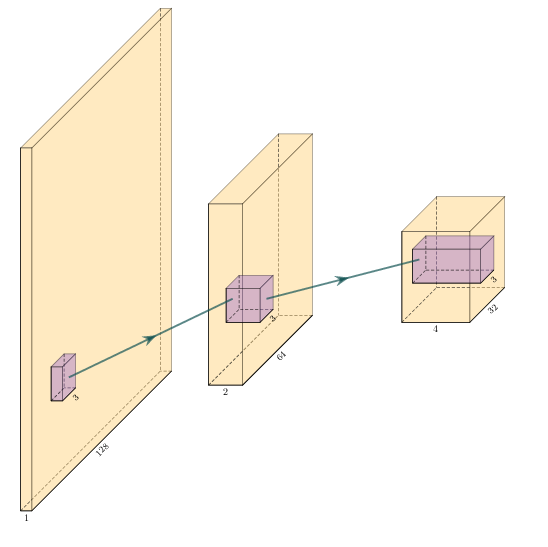
Figure 7.2: Schematic convolutional neural network. The input layer (yellow) is convolved with a \(3\times3\) filter that results in a spatially subsampled subsequent layer that contains the filter responses. This second layer is again convolved with a \(3\times3\) filter to obtain the next layer. Subsampling is achieved by strided convolutions or pooling.
CNNs are a type of neural network that is particularly suited to imaging approaches. They learn arbitrary data-dependent filters that are optimized based on the chosen objective via gradient descent. These filters can operate on real images, medical images, or seismic data alike. The convolutional filter benefits from weight sharing, making the operation efficient and particularly suited to GPUs or specialized hardware. In Figure 7.2 we show a schematic image, that is convolved with moving 3x3 filters repeatedly to obtain a spatially downsampled representation. These convolutional layers in neural networks can be arranged in different architectures that we explore in the following analysis of prior methods in image alignment.
Supervised convolutional neural networks
Supervised end-to-end convolutional neural networks rely on reliable ground truth, including the time shifts being available. Training a supervised machine learning system requires both a data vector \(x\) and a target vector \(y\) to train the blackbox system \(f(x) \Rightarrow y\). This means that we have to provide extracted time-shifts from other methods, which implicitly introduce assumptions from that method into the supervised model. Alternatively, expensive synthetic models would be required.
The supervised methods are largely based on Optical Flow methods (Dosovitskiy et al. 2015; Ranjan and Black 2017). The FlowNet (Dosovitskiy et al. 2015) architecture is based on an Encoder-Decoder CNN architecture. Particularly, FlowNet has reached wide reception and several modifications were implemented, namely FlowNet 2.0 (Ilg et al. 2017) improving accuracy, and LiteFlowNet (Hui, Tang, and Change Loy 2018) reducing computational cost. SpyNet (Ranjan and Black 2017) and PWC-Net (D. Sun et al. 2018) implement stacked coarse-to-fine networks for residual flow correction. PatchBatch (Gadot and Wolf 2016) and deep discrete flow (Güney and Geiger 2016) implement Siamese Networks (Sumit Chopra et al. 2005) to estimate optical flow. Alternatively, DeepFlow (Weinzaepfel et al. 2013) attempts to extract large displacements optical flow using pyramids of SIFT features. These methods introduce varying types of network architectures, optimizations, and losses that attempt to solve the optical flow problem in computer vision.
Unsupervised convolutional neural networks
Unsupervised or self-supervised convolutional neural networks only rely on the data, relaxing the necessity for ground truth time shifts. In (Meister, Hur, and Roth 2018) the FlowNet architecture is reformulated into an unsupervised optical flow estimator with bidirectional census loss called UnFlow. The UnFlow network relies on the smooth estimation of the forward and backward loss, then adds a consistency loss between the forward and backward loss and finally warps the monitor to the base image to obtain the final data loss. Optical flow has historically underperformed on seismic data, due to both smoothness and illumination constraints. However, UnFlow replaces the commonly used illumination loss by a ternary census loss (Zabih and Woodfill 1994) with the \(\epsilon\)-modification by (Stein 2004). While this bears possible promise for seismic data, UnFlow implements 2D losses as opposed to a 3D implementation that we focus on.
Cycle-consistent Generative Adversarial Networks
Cycle-GANs are a unsupervised implementation of Generative Adversarial Networks that are known for domain adaptation (J.-Y. Zhu et al. 2017). These implement two GAN networks that perform a forward and backward operation that implements a cycle-consistent loss in addition to the GAN loss. The warping problem can be reformulated as a domain adaptation problem. This implements two Generator networks \(F\) and \(G\) and the according discriminators \(D_X\) and \(D_Y\). These perform a mapping \(G: X \rightarrow Y\) and \(F: Y \rightarrow X\), trained via the GAN discrimination. The cycle-consistency implements \(x \rightarrow G(x) \rightarrow F(G(x)) \approx x\) with the backwards cycle-consistency being \(y \rightarrow F(y) \rightarrow G(F(y)) \approx y\).
Cycle-GANs such as pix2pix (Isola et al. 2017) separate image data into a content vector and a texture vector, which could bear promise in the seismic domain, adapting a wavelet vector and an interval vector (Lukas Mosser, Kimman, Dramsch, Purves, De la Fuente Briceño, et al. 2018). However, the confounding of imaging effects, changing underlying geology, changing acquisition, etc makes the separation non-unique. Moreover, extracting the time shift information and conditioning in the GAN is a very complex problem. The Recycle-GAN (Bansal et al. 2018) addresses temporal continuity in videos, this is however hard to transfer to seismic data, considering the low number of time-steps in a 4D seismic survey as opposed to videos. Furthermore, the lack of interpretability of GANs at the point of writing, prohibits GANs from replacing many physics-based approaches, like the extraction of time-shifts.
Method
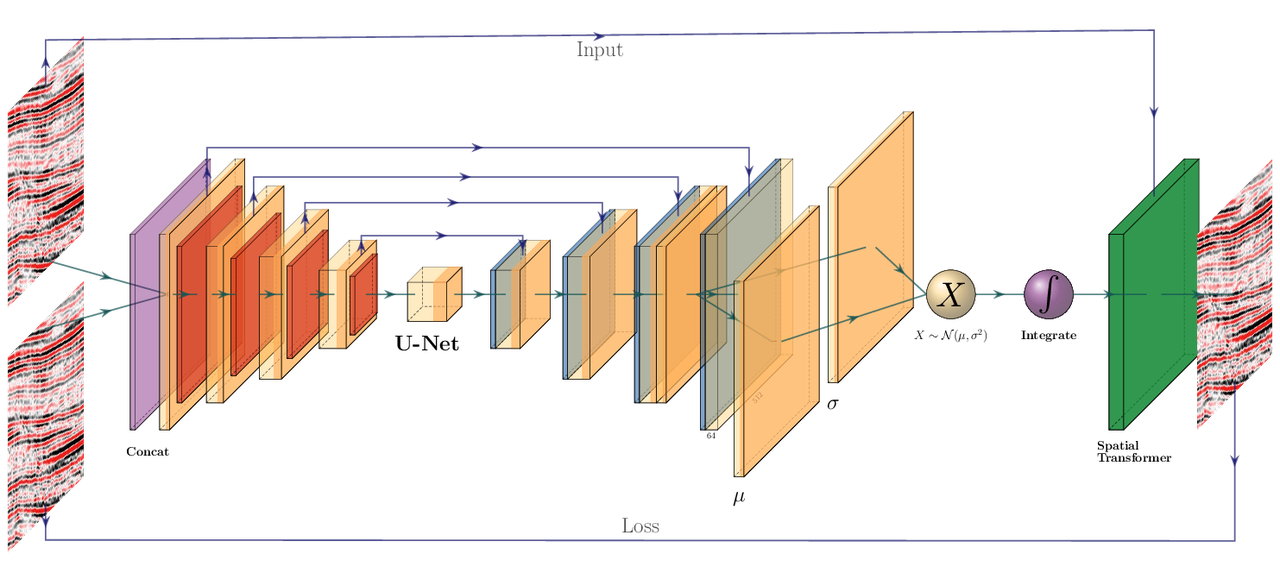
Figure 7.3: 2D representation of Modified 3D Voxelmorph architecture to obtain full scale warp velocity field. The Encoder side of the U-Net architecture consists of four consecutive Convolutional (orange) and Pooling (red) layers, followed by a convolutional Bottleneck layer. The decoder of the U-Net architecture consists offour Upsampling (blue) and Convolutional layers are connected to the respective same size layers in the Encoder. The output is passed to two convolutional layers that are sampled by the reparametrization trick, to provide the static velocity field. The field is integrated via scaling and squaring and passed to the Spatial Transformer layer (green), which transforms the monitor to optimally match the base image, which is enforced by minimizing the mean squared error (MSE) of the images.
The Voxelmorph (Balakrishnan et al. 2019) implements a U-net (Ronneberger, Fischer, and Brox 2015b) architecture to obtain a dense warp velocity field and subsequently warps the monitor volume to match the base volume. This minimizes assumptions that have to be satisfied for applying optical flow-based methods. Additionally, the Voxelmorph architecture was specifically developed on medical data. Here we use an advancement of Voxelmorph that includes a variational layer, which introduced uncertainty to the static velocity estimation, developed in (Dalca, Balakrishnan, Guttag, et al. 2018). Medical data often has fewer samples, like seismic data, as opposed to popular video datasets, which FlowNet and derivative architectures are geared towards application of popular video datasets. A U-net architecture is particularly suited for segmentation tasks and transformations with smaller than usual amounts of data, considering it was introduced on a small biomedical dataset. The short-cut concatenation between the input and output layers stabilizes training and avoids the vanishing gradient problem. It is particularly suited to stable training in this image matching architecture. In Figure 7.3 the U-Net is the left-most stack of layers, aranged in an hourglass architecture with shortcuts. These feed into a variational layer \(\mathcal{N(\mu,\sigma)}\), the variational layer is sampled with the reparametrization trick, due to the sampler not being differentiable (Durk P. Kingma, Salimans, and Welling 2015). The resulting differential flow is integrated using the VecInt layer, which uses Scaling and Squaring (Higham 2005). Subsequently, the data is passed into a spatial transformation layer. This layer transforms the monitor cube according to the warp velocity field obtained from the integrated sampler. The result is used to calculate the data loss between the warped image and the base cube.
More formally, we define two 3D images \(\bf{b, m}\) being the base and monitor seismic respectively. We try to find a deformation field \(\phi\) parameterized by the latent variable \(z\) such that \(\phi_z: \mathbb{R}^3 \rightarrow \mathbb{R}^3\). The deformation field itself is defined by this ordinary differential equation (ODE) according to (Balakrishnan et al. 2019):
where \(t\) is time, \(v\) is the stationary velocity and the following holds true \(\phi^{(0)} = \bf{I}\). The integration of \(v\) over \(t=[0,1]\) provides \(\phi^{(1)}\). This integration represents and implements the one-parameter diffeomorphism in this network architecture. The variational Voxelmorph formulation assumes an approximate posterior probability \(q_\psi(z|\bf{b};\bf{m})\), with \(\psi\) representing the parameterization. This posterior is modeled as a multivariate normal distribution with the covariance \(\Sigma_{z|m,b}\) being diagonal:
the effects of this assumption are explored in (Dalca, Balakrishnan, Guttag, et al. 2018).
The approximate posterior probability \(q_\psi\) is used to obtain the variational lower bound of the model evidence by minimizing the Kullback-Leibler (KL) divergence with \(p(z|\bf{b};\bf{m})\) being the intractable posterior probability. Following the full derivation in (Dalca, Balakrishnan, Guttag, et al. 2018), considering the sampling of \(z_k \sim q_\psi(z|\bf{b},\bf{m})\) for each image pair \((\bf{b},\bf{m})\), we compute \(\bf{m}\circ\phi_{z_k}\) the warped image we obtain the loss:
where \(\Lambda_z\) is a precision matrix, enforcing smoothness by the relationship \(\Sigma_z^{-1} = \Lambda_z = \lambda \bf{L}\), \(\lambda\) controlling the scale of the velocity field. Furthermore, following (Dalca, Balakrishnan, Guttag, et al. 2018) \(\bf{L} = \bf{D} - \bf{A}\) is the Laplacian of a neighbourhood graph over the voxel grid, where \(\bf{D}\) is the graph degree matrix, and \(A\) defining the voxel neighbourhood. \(K\) signifies the number of samples. We can express \(\bf{\mu}_{z|m,b}\) and \(\Sigma_{z|m,b}\) as variational layers in a neural network and sample from the distributions of these layers. Given the diagonal constraint on \(\Sigma\), we define the variational layer as the according standard deviation \(\sigma\) of the corresponding dimension. Therefore, we sample \(\mathcal{X} \sim \mathcal{N}(\mu, \sigma^2)\) using the reparameterization trick first implemented in variational auto-encoders (Diederik P. Kingma and Welling 2013). The reparameterization trick defines a differentiable estimator for the variational lower bound, replacing the stoachastic, non-differentiable and therefore untrainable, sampler.
Defining the architecture and losses as presented in (Dalca, Balakrishnan, Guttag, et al. 2018), ensures several benefits. The registration of two images is domain-agnostic, which enables us to apply the medical algorithm to seismic data. The warp field is diffeomorphic, which ensures physically viable, topology-preserving warp velocity fields. Moreover, this method implements a variational formulation based on the covariance of the flow field. 3D warping with uncertainty measure has not been used in seismic data before.
The network is implemented using Tensorflow (Abadi et al. 2015a) and Keras (Chollet and others 2015a). Our implementation is based on the original code in the Voxelmorph package (Dalca, Balakrishnan, Fischl, et al. 2018).
Experimental Results and Discussion
Experimental Setup
The experimental setup for this paper is based on a variation of the modified Voxelmorph (Balakrishnan et al. 2019) formulation. We extended the network to accept patches of data, because our seismic cubes are generally larger than the medical brain scans and therefore exceed the memory limits of our GPUs. Moreover, Voxelmorph in its original formulation provides sub-sampled flow fields, this is due to computational constraints. We decided to modify the network to provide full-scale flow fields, despite the computational cost. This enables direct interpretation of the warp field, which is common in 4D seismic analysis. However, we do provide an analysis in Section 7.4.4.2 of the sub-sampled flow-field interpolated to full scale, in the way it would be passed to the Spatial Transformer layer.
The code is made available in (Jesper Soeren Dramsch 2020c). The model is trained with the Adam optimizer (Diederik P. Kingma and Ba 2014) with a learning rate of \(0.001\) and weight decays \(\beta_1 = 0.9\) and \(beta_2 = 0.999\). We train the model for 350 epochs to account for experimentation and time. We set the regularization parameter \(\lambda = 10\) and the image noise parameter \(\sigma = 0.02\) in accordance with the authors of (Dalca, Balakrishnan, Guttag, et al. 2018). We adjust the batch-size to the maximum on our architecture, which was 16 and purely manually tuned to the maximum possible. The KL divergence and MSE loss are unweighted in the total loss.
The network definition for the subsampled flow field differs from the definition in Figure 7.3 that the last upsampling and convolution layer in the Unet, including the skip connection, right before the variational layers \((\mu, \sigma)\) is omitted. That leaves the flow field at a subsampled map by a factor of two. Computationally, this lowers the cost on the Integration operation before resampling for the Spatial Transformer.
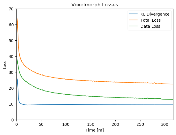
Figure 7.4: Training Losses over time with the KL-divergence at the sampling layer, the data loss calculated by MSE, and the combined total loss.
The data situation for this experiment is special in the sense that the method is self-supervised. We therefore do not provide a validation dataset during training. The data are 6 surveys from the North Sea. Main field from years 1088, 2005 A, 2005 B, and 2012. Further we compare to a different field 1903 and 2005 with different geology, acquisition geometry and acquisition parameters. While we would be content with the method working on the field data (years 1988 and 2005 Survey A) by itself, we do validate the results on separate data from the same field which was acquired with different acquisition parameters and at different times (years 2005 Survey B and 2012). Moreover, we test the data on seismic data from an adjacent field that was acquired independently (years 1993 and 2005). All data is presented with a relative coordinate system due to confidentiality, where 0 s on the y-axis does not represent the actual onset of the recording. The field geology and therefore seismic responses are very different. Due to lack of availability we do not test the trained network on land data or data from different parts of the world. Considering, that the training set is one 4D seismic monitor-base pair, a more robust network would emerge from training on a variety of different seismic volumes.
Figure 7.4 shows the training losses of the batch training. Within a few epochs the network converges strongly, however within 10 epochs the KL divergence increases slightly over the training. The data loss, optimizing the warping result decreases over the training period. An increase of the KL divergence is acceptable as long as the total loss decreases, which indicates better matching of the volumes. In case the KL divergence would increase vastly, it would violate the base assumption that the static velocity can be approximated by Gaussians and requires re-evaluation.
Results and Discussion
The network presented generates warp fields in three dimensions as well as uncertainty measures. We present results for three cases in Figure 7.5, Figure 7.10, and Figure 7.12 with the corresponding warp fieds and uncertainties in Figure 7.6, Figure 7.11, and Figure 7.13. In Figure 7.5 we show the results on the data, which the unsupervised method was trained on. Obtaining a warp field on the data itself is a good result, however, we additionally explore the generalizability of the method. Considering the network is trained to find an optimum warp field for the data it was originally trained on, we go on to test the network on data from the same field, that was recorded with significantly different acquisition parameters in Figure 7.10. These results test the networks generalizability on co-located data, therefore not expecting vastly differing seismic responses from the subsurface itself. The are imaging differences and differences in equipment in addition to the 4D difference however. In Figure 7.12 we use the network on unseen data from a different field. The geometry of the field, as well as the acquisition parameters are different, making generalization a challenge.
|
|
|
|
|
|
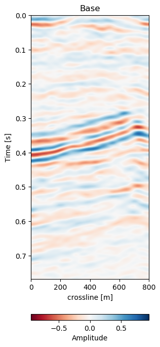
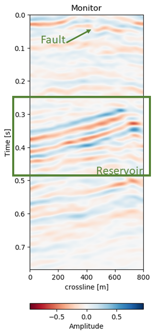
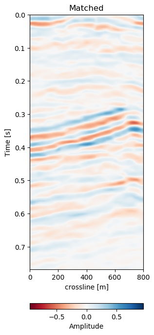
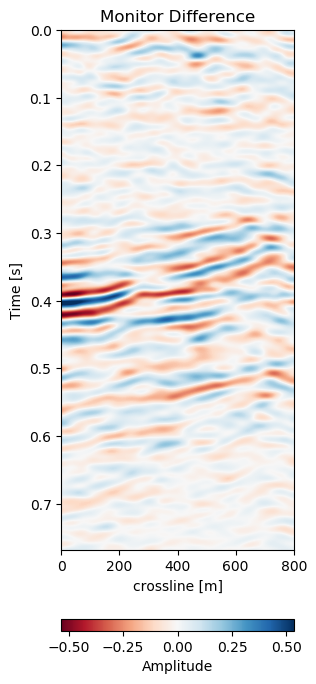
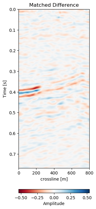
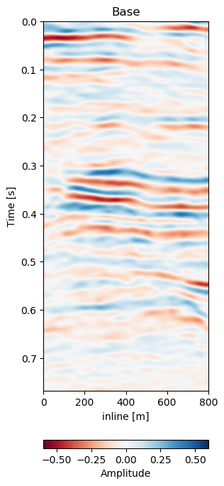
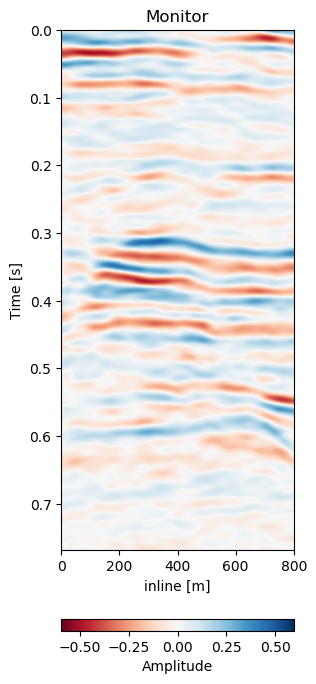
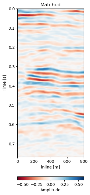
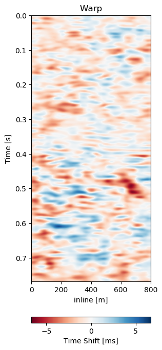
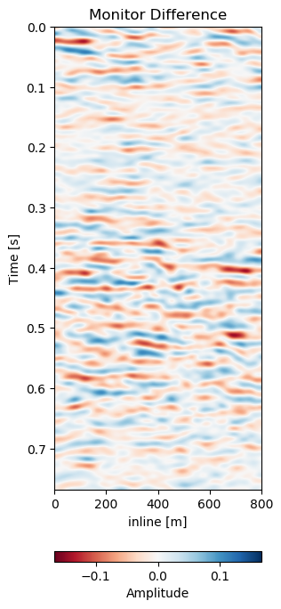
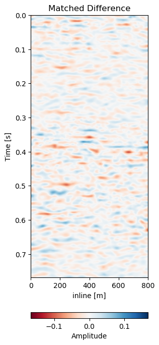
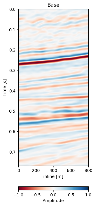
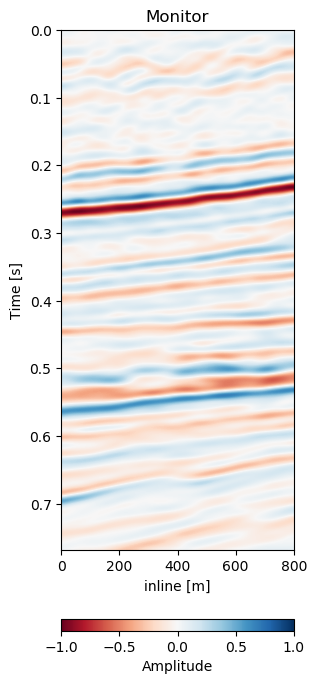
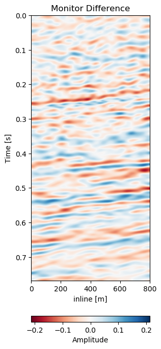
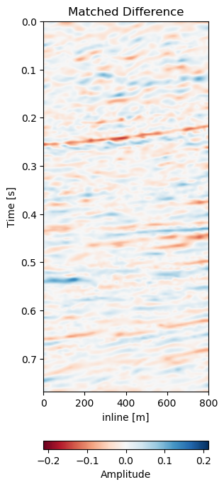
Figure 7.5: Warp results and change in difference on training recall of 1988 to 2005a data. Axes are relative to comply with confidentiality..
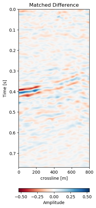
In Figure 7.5 we collect six 2D panels from the 3D warping operation. In Figure 7.5 (a) and Figure 7.5 (b) we show the unaltered base and monitor respectively. The difference between the unaltered cubes is shown in Figure 7.5 (e). In Figure 7.5 (c) we show the warped result by applying the z-warp field in Figure 7.5 (d), as well as the warp fields in (x,y) direction fully displayed in Figure 7.6 including their respective uncertainties. The difference of the warped result in Figure 7.5 (f) is calculated from the matched monitor in Figure 7.5 (c) and the base in Figure 7.5 (a).
It is apparent that the matched monitor significantly reduced noise by mis-aligned reflections. In Table 7.1 we present the numeric results. These were computed on the 3D cube for an accurate representation. We present the root mean square (RMS) and mean absolute error (MAE) and the according difference between Monitor and Matched Difference results. We present RMS and MAE to make the values comparable in magnitude as opposed the mean squared error (MSE). We present both values, because the RMS value is more sensitive to large values, while MAE scales the error linearly therefore not masking low amplitude mis-alignments. Both measurements show a reduction on the train data to 50% or below. The test on both the validation data on the same field and the test data on another field show a similar reduction, while the absolute error differs in a stable manner.
Run |
Monitor RMS |
Matched RMS |
Ratio % |
Monitor MAE |
Matched MAE |
Ratio % |
Baseline |
0.1047 |
0.0718 |
68.6 |
0.0744 |
0.0512 |
68.7 |
Train |
0.1047 |
0.0525 |
50.1 |
0.0744 |
0.0348 |
46.7 |
Test A |
0.0381 |
0.0237 |
62.2 |
0.0291 |
0.0172 |
59.1 |
Test B |
0.0583 |
0.0361 |
62.0 |
0.0451 |
0.0254 |
56.4 |
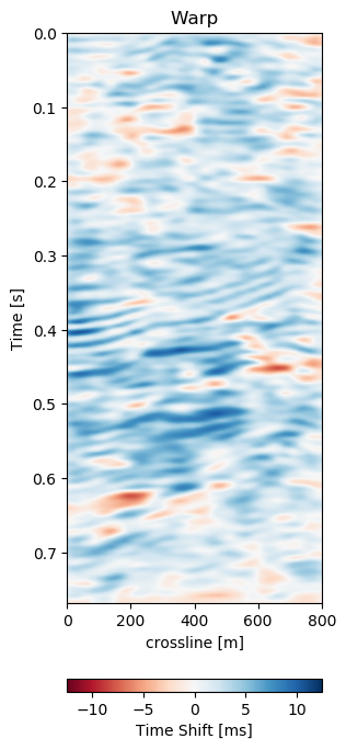
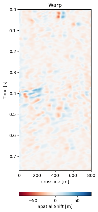
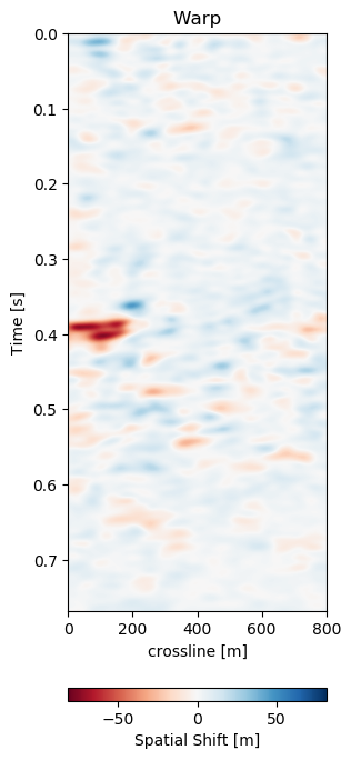
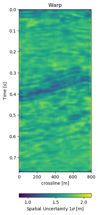
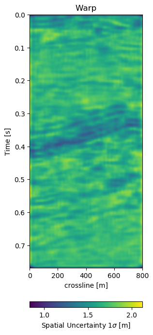
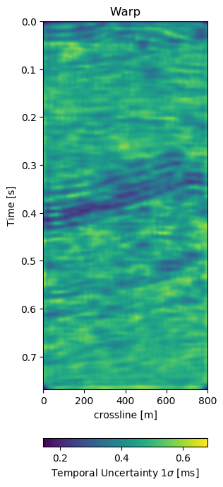
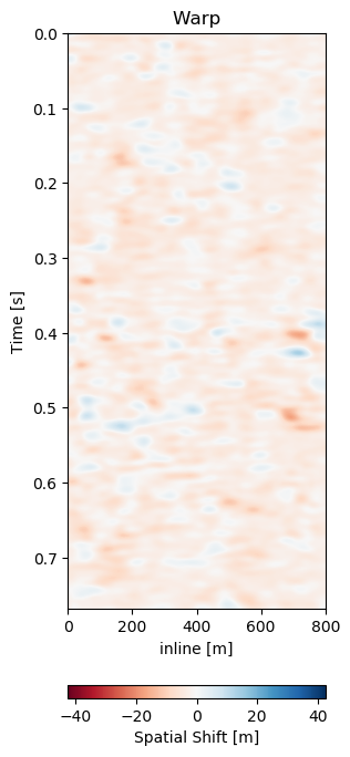
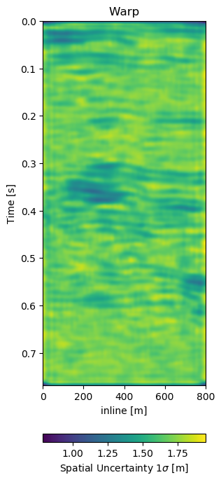
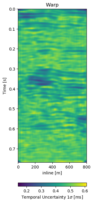
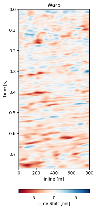
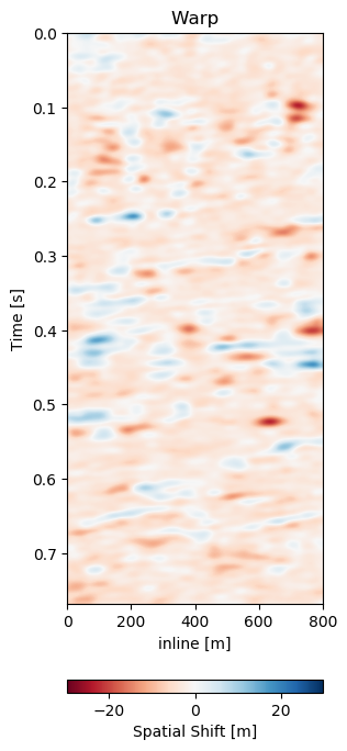
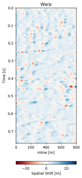
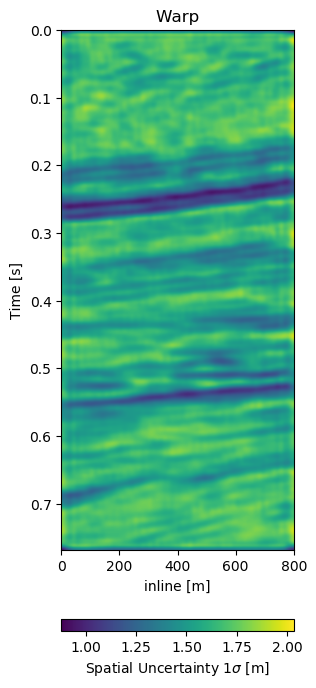
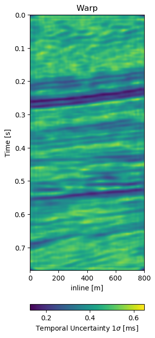
In Figure 7.6 we present the three dimensional warp field to accompany the results in Figure 7.5. Figure 7.6 (a), Figure 7.6 (b), and Figure 7.6 (c) show the warp field in x, y, and z-direction. The z-direction is generally referred to as time shifts in 4D seismic. Figure 7.6 (d), Figure 7.6 (e), and Figure 7.6 (f) contain the corresponding uncertainties in x, y, and z-direction obtained from the network.
|
|
|
|
|
|
Figure 7.6: Warp fields (top) with uncertainties (bottom) that accompanies training recall in Figure 7.5.
Recall to Training Data
In Figure 7.5 we evaluate the results of the self-supervised method on the training data itself. The main focus is on the main reflector in the center of the panels. The difference in Figure 7.5 (e) shows that the packet of reflectors marked reservoir in the monitor is out of alignment, causing a large difference, which is corrected for in Figure 7.5 (f). The topmost section in the panel of Figure 7.5 (c) shows the alignment of a faulted segment, marked fault in the monitor, to an unfaulted segment in the base. The fault appearing is most likely due to vastly improved acquisition technology for the monitor.
The warp fields in Figure 7.6 are an integral part in QC-ing the validity of the results. Physically, we expect the strongest changes in the z-direction in Figure 7.6 (c). The changes in Figure 7.6 (a) and Figure 7.6 (b) show mostly sub-sampling magnitude shifts, except for the x-direction shifts around the fault in the top-most panel present in the monitor in Figure 7.5 (b). Figure 7.6 (a) and Figure 7.6 (b) show strong shifts at 0.4s on the left of the panel which corresponds to the strong amplitude changes in the base and monitor. On the one side these correspond to the strongest difference section, additionally these are geological hinges, which are under large geomechanical strain. However, these are very close to the sides of the warp, which may cause artifacts. Figure 7.6 (d), Figure 7.6 (e), and Figure 7.6 (f) show the uncertainty of the network. These uncertainties are across the bank within the 10% range of the sampling rate (\(\Delta t = 4\) ms, \(\Delta x,y = 25\) m). The certainty within the bulk package in the center of the panels is the lowest in x-, y-, and z-direction. While being relatively lover in the problematic regions discussed before.
The warp field in Figure 7.6 (d) contains some reflector shaped warp vectors around 0.4 s, which is due to the wavelet mismatch of the 1988 base to the 2005 monitor. The diffeomorphic nature of the network aligns the reflectors in the image, which causes some reflector artifacts in the z-direction maps.
Comparison to Baseline Method
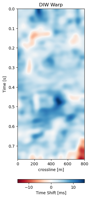
We use the Dynamic Image Warping method (Dave Hale 2013a) to align the images in Figure 7.5. This method extends the Dynamic Time Warping method to 2D and provides a much improved result in 2D compared to standard cross-correlation and DTW methods. Inversion methods need pre-stack seismic data, which is not available. We chose this baseline to provide a fair comparison with the available data. Figure 7.7 shows the timeshifts or warp fields generated by the Voxelmorph network and by the DIW algorithm. The DIW algorithm shows a smoothed image. Overall, the Subfigre 7.7 (b) shows the general trends of Subfigre 7.7 (a). The Voxelmorph algorithm is more detailed than the DIW image, however the general magnitude of the time shifts matches well in the correct areas.
|
|
Figure 7.7: Comparison of Voxelmorph warp field (left) and Dynamic Image Warping (right) warp fields.
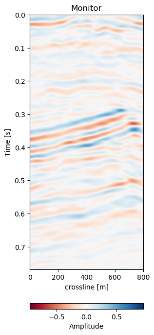
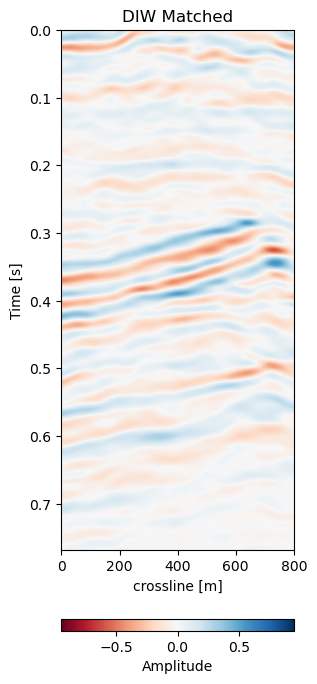
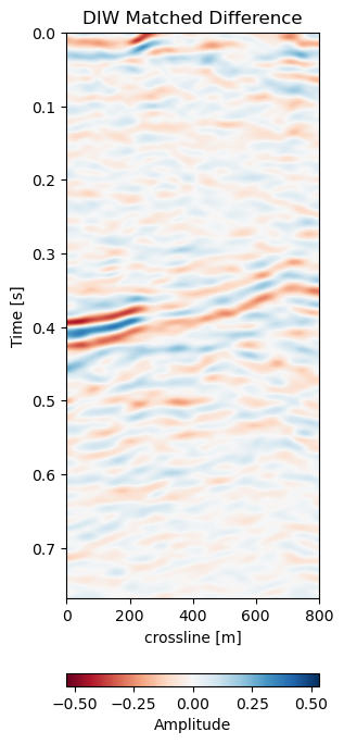
Figure 7.8 shows the matched monitors from Voxelmorph and DIW. The matched monitors align quite well without any significant discrepancies. The matched difference shows that the Voxelmorph algorithm performs similarly to the baseline method, while removing more 4D noise from the image. It keeps the 4D signal intact, albeit slightly varying. The DIW algorithm seems to struggle to align the topmost part of the image, while Voxelmorph aligns these well, removing additional 4D noise. Table 7.1 confirms this quantitatively, where the overall RMSE and MAE are reduced proportionally.
|
|
|
|
|
|
Figure 7.8: Results of Voxelmorph warping compared to baseline dynamic image warping algorithm. Top row shows the aligned monitor, bottom row shows the difference to the base volume.
Generalization of the Network
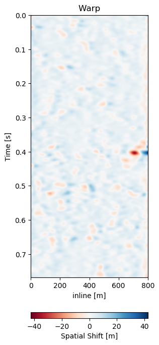
While the performance of the method on a data set by itself is good, obtaining a trained model that can be applied on other similar data sets is essential even for self-supervised methods. We test the network on two test sets, Test A is conducted on the same geology with unseen data from a different acquisition, while Test B is on a different field and a different acquisition. The network was trained on a single acquisition relation (2005a - 1988). In Figure 7.10 we present the crossline data from the same field the network was trained on. The data sets was however acquired at a different calendar times (2005b - 2012), with different acquisition parameters. It follows that although the geology and therefore the reflection geometry is similar, the wavelet and hence the seismic response are vastly different. This becomes apparent when comparing the base Figure 7.10 (a) to Figure 7.5, which were acquired in the same year.
|
|
|
|
|
|
Figure 7.10: Matched difference and warp field for generalization of network to same field with different data (2005b and 2012).
Test A evaluates the network performance on unseen data in the same field (Train: 1988-2005a, Test A: 2005b - 2012). The quantitative results in Table 7.1 for Test A generally show lower absolute errors compared to the training results in Section 7.4.4.2. The reduction of the overall amplitudes in the difference maps is reduce by 40%. The unaligned monitor difference in Figure 7.10 (e) shows a strong coherent difference around below the main packet of reflectors around 0.3 s to 0.4 s. This would suggest a velocity draw-down in this packet. While the top half of the unaligned difference contains some misalignment, we would expect the warp field to display a shift around 0.35 s, which can be observed in Figure 7.10 (d). The aligned difference in Figure 7.10 (f) contains less coherent differences. The difference does still show some overall noise in the maps. This could be improved upon by a more diverse training set. The higher resolution data from 2005 and 2012 possibly has an influence on the result too. Regardless, we can see some persisting amplitude difference around 0.4 s which appears to be signal as opposed to some misalignment noise above. The warp fields in Figure 7.11 show relatively smooth warp fields in x- and y-direction. The warp field in Figure 7.11 (f) shows overall good coherence, including the change around 0.4 s we would expect. The uncertainty values are in sub-sampling range, with the strongest certainty within the strong reflector packet at 0.35 s.
|
|
|
|

|
|
Figure 7.11: Warp fields (top) with uncertainties (bottom) that accompanies same field generalization in Figure 7.10.
Test B evaluates the network performance on a different field, with different geology, with unrelated acquisition geometry and equipment and at different times. The test shows a very similar reduction of overall errors in Table 7.1. The RMS is reduced by 38% and the MAE is reduced more slightly more in comparison to Test A. In Figure 7.12 we present the seismic panels to accompany Test B. The data in Figure 7.12 (a) and Figure 7.12 (b) is well resolved and shows good coherence. However, the unaligned difference in Figure 7.12 (e) shows very strong variations in the difference maps. Figure 7.12 (f) reduces these errors significantly, bringing out coherent differences in the main reflector at 0.27 s. We can see strong chaotic differences in Figure 7.12 (e), due to the faulted nature of the geology. The network aligns these faulted blocks relatively well, however, some artifacts persist. This is consistent with the warp fields in Figure 7.13. The x- and y-direction in Figure 7.13 (d) and Figure 7.13 (e) respectively show overall smooth changes, around faults, these changes are stronger. The z-direction changes are consistent with the Training validation and Test A, where the changes are overall stronger. This is also consistent with our geological intuition.
|
|

|
|
|
|
Figure 7.12: Matched difference and warp field for generalization of network to a different field (1993 and 2005).
|
|
|

|
|
|
Figure 7.13: Warp fields (top) with uncertainties (bottom) that accompanies different field generalization in Figure 7.12.
Subsampled Flow
The original Voxelmorph implementation uses a subsampled warp field. The authors claim two benefits, namely a smoother warp velocity field and reduced computational cost. The aforementioned results were obtained using our full-scale network. In Figure 7.9 we present the full scale and upsampled results on the training set. The matched difference in Figure 7.9 (b) contains more overall noise compared to Figure 7.9 (a). This is congruent with the warp fields in the figure. The upsampled z-direction warp field in Figure 7.9 (d) seems to have some aliasing on the diagonal reflector around 0.4 s. This explains some of the artifacts in the difference in Figure 7.9 (b). The overall warp velocity in Figure 7.9 (d) is smoother compared to the full-scale field. However, the general structure of coherent negative and positive areas matches in both warp fields, while the details differ. The main persistent difference of the reflector packet at 0.4 s seems similar, nevertheless, the differences further up slope to the right are smoother in the full scale network result and have stronger residual amplitudes in the upsampled network. Overall, the full-scale network results are better for seismic data at a slightly increased computational cost. The subsampled field introduced artifacts in our observations.
|
|
|
|
Figure 7.9: Comparison of matched differences (top) and z-direction warp field (bottom) of full-scale neural architecture (left) and subsampled neural architecture (right).
Conclusion
We introduce a deep learning based self-supervised 4D seismic warping method. Currently, time shifts are most commonly estimated in 1D due to computational constraints. We explore 3D time-shift estimation as a viable alternative, which decouples imaging and acquisition effects, geomechanical movement and changes in physical properties like velocity and porosity from confounding into a single dimension. Existing 3D methods are computationally expensive, where this learnt model can generalize to unseen data without re-training, with calculation times within minutes on consumer hardware. Moreover, this method supplies invertible, reproducible, dense 3D alignment while providing warp fields with uncertainty measures, while leveraging recent advancements in neural networks and deep learning.
We evaluate our network on the training data and two different independent test sets. We do not expect the aligned difference to be exactly zero, due to actual physical changes in the imaged subsurface. Although the network is unsupervised, a transfer to unseen data is desirable and despite some increase in the overall error possible. The warping on the training data is very good and the warp fields are coherent and reflect the physical reality one would expect. The transfer too unseen data works well, although the misalignment error increases. The decrease in both RMS and MAE is consistent across test sets.
Furthermore, we implement a variational scheme which provides uncertainty measures for the time shifts. On the data presented, we obtain subsample scale uncertainties across all directions. The main assumption of the network is a diffeomorphic deformation, which is topology preserving. We show that the network handles faults well in both training recall and test data, that in theory could violate the diffeomorphic assumption.
We go on to compare a full-scale network to an upsampled network. The full-scale network yields better results and is preferable on seismic data in comparison to the upsampled network presented in the original medical Voxelmorph.
We do expect the network to improve upon training on a more diverse variety of data sets and seismic responses. While the initial training is time-consuming (25 h on a Nvidia Titan X with Pascal chipset), inference is near instantaneous. Moreover, transfer of the trained network to a new data set is possible without training, while accepting some error. Alternatively fine-tuning to new data is possible within few epochs (\(<\)1 h).
Acknowledgment
The research leading to these results has received funding from the Danish Hydrocarbon Research and Technology Centre under the Advanced Water Flooding program. We thank DTU Compute for access to the GPU Cluster. We thank Total E&P Denmark for permission to use the data and publish examples.
Contributions of This Study
In the paper, we present the modified self-supervised neural network system and test the results on the training data itself and two generalization test sets. The first test set is on the same field but recorded at different times to the training set, ensuring similar underlying geology, whereas, the second test set is taken from an adjacent field, recorded at different times, with different geology, testing the full transfer of the trained network. We go on to test the original Voxelmorph architecture, which uses upsampled velocity fields and evaluate the results against our modified architecture, which uses the full flow field. Overall, this technique introduces a generalizable dl approach to extract 3D time-shifts with uncertainty measures from raw stacked 4D seismic data.
The Voxelmorph network performs very well on seismic data with patch-based seismic data. It is essential to implement the full-scale architecture to obtain reliable 3D time-shifts on 4D seismic data. The network exhibits stable error on the unseen data on the same field and differing test field, which indicates that the networks learn relevant generalizable information. Despite being a 3D method, the primary shifts are estimated in the z-direction, which is consistent with the expectation we have for seismic data. The diffeomorphic assumption performs well on the seismic data even on faulted data, preserving the topology. Additionally, unsupervised training reduces further implicit assumptions from extracted time-shifts or synthetic models. The model would improve from data augmentation methods and including multiple fields in the training data.